← All Chapters
Summary Note 5 / 7

Chapter 5 – Pumping Test & Aquifer Parameter Estimation

GWE Handwritten Notes

Page 49

Page 49
Transcription

Chapter 5 – Pumping Test Methods

Ground Surface Confined Aquifer Original Piezometric Surface Pumping Well ⬆ Q Cone of Depression OW₁ s₁ OW₂ r₁ r₂ b
Fig: Pumping test setup showing cone of depression in a confined aquifer

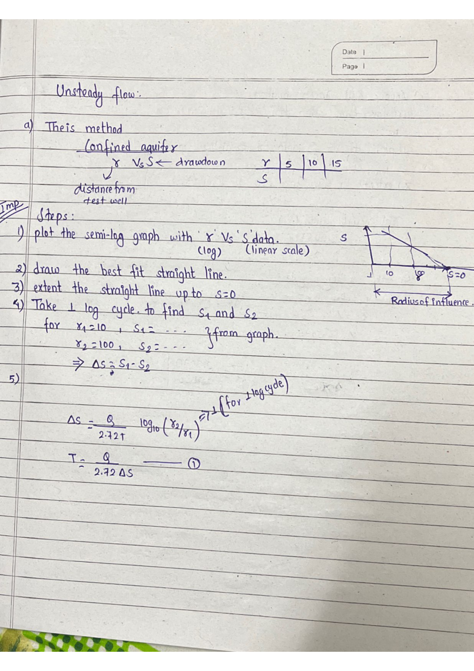
a) Theis Method (Distance-Drawdown)

Confined aquifer

Steps:

  1. Plot r vs s in semi-log graph (r → log, s → linear)
  2. Draw best fit straight line
  3. Extend to s = 0 → Radius of Influence (R0)
  4. Take 1 log cycle: Δs = s1 − s2
  5. T:
    \( T = \frac{2.303\,Q}{2\pi\,\Delta s} = \frac{Q}{2.72\,\Delta s} \)

Page 50

Page 50
Transcription

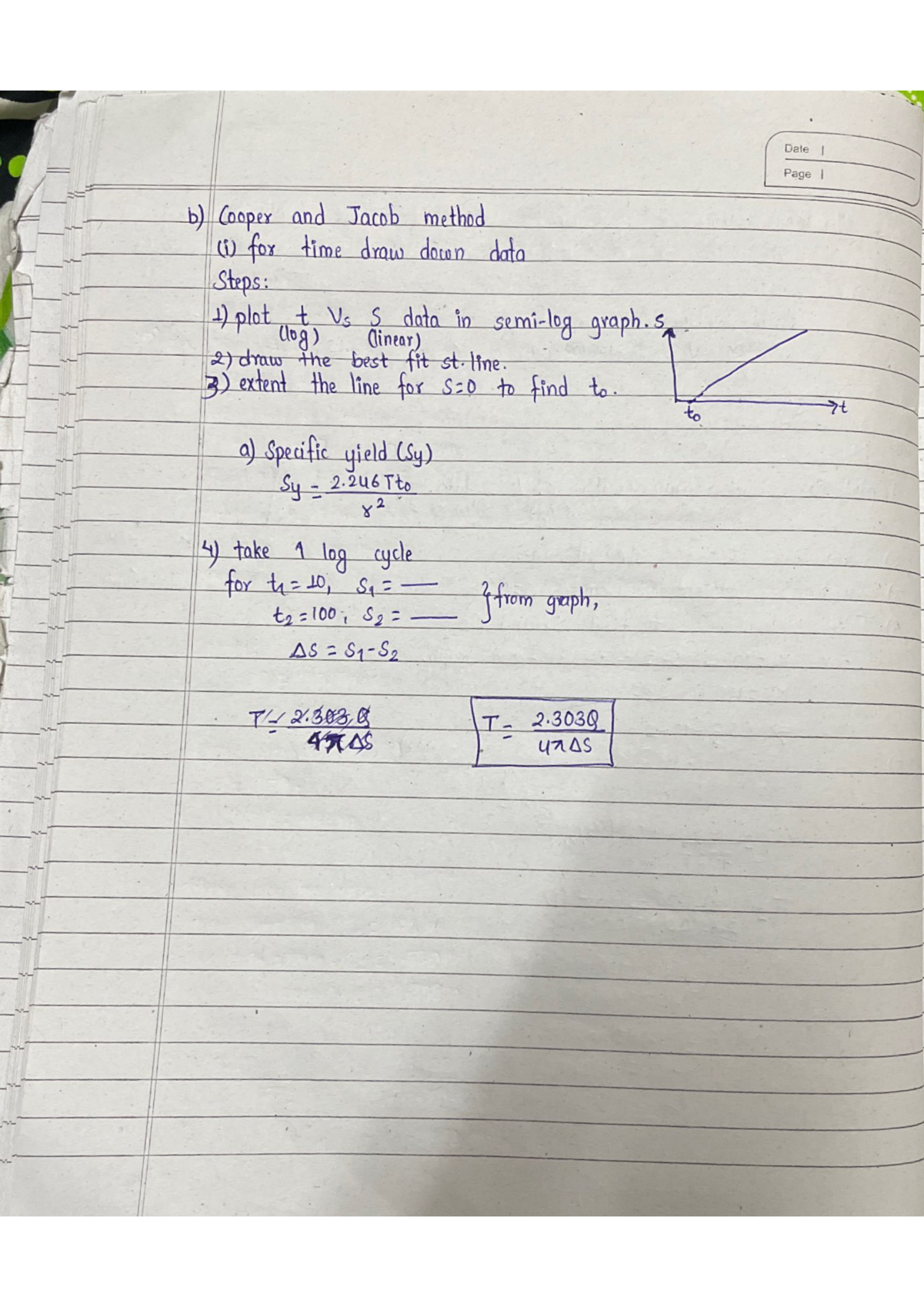
b) Cooper and Jacob Method (Time-Drawdown)

Steps:

  1. Plot t vs s in semi-log graph (t → log, s → linear)
  2. Draw best fit straight line
  3. Extend to s = 0 → find t0
  4. Take 1 log cycle: Δs = s2 − s1
\( T = \frac{2.303\,Q}{4\pi\,\Delta s} \)
\( S_y = \frac{2.246\,T\,t_0}{r^2} \)

Page 51

Page 51
Transcription

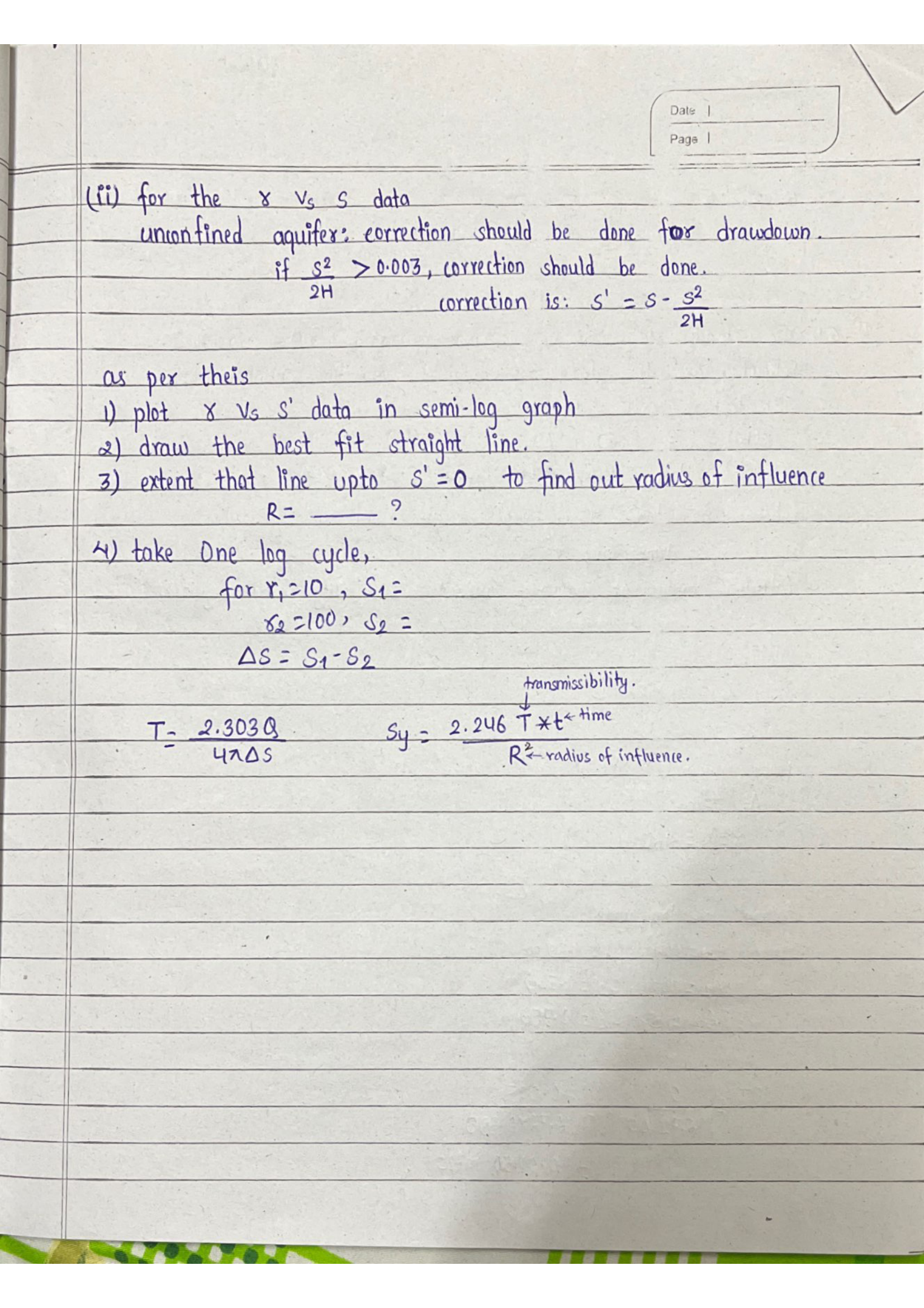
Unconfined Aquifer Correction

If s²/(2H) > 0.003, correction required:

\( s' = s - \frac{s^2}{2H} \)

Then use corrected s′ in same semi-log method:

\( T = \frac{2.303\,Q}{4\pi\,\Delta s'} \)
\( S_y = \frac{2.246\,T\,t_0}{R^2} \)

Page 52

Page 52
Transcription

Chapter 5 – Pumping Test Numericals

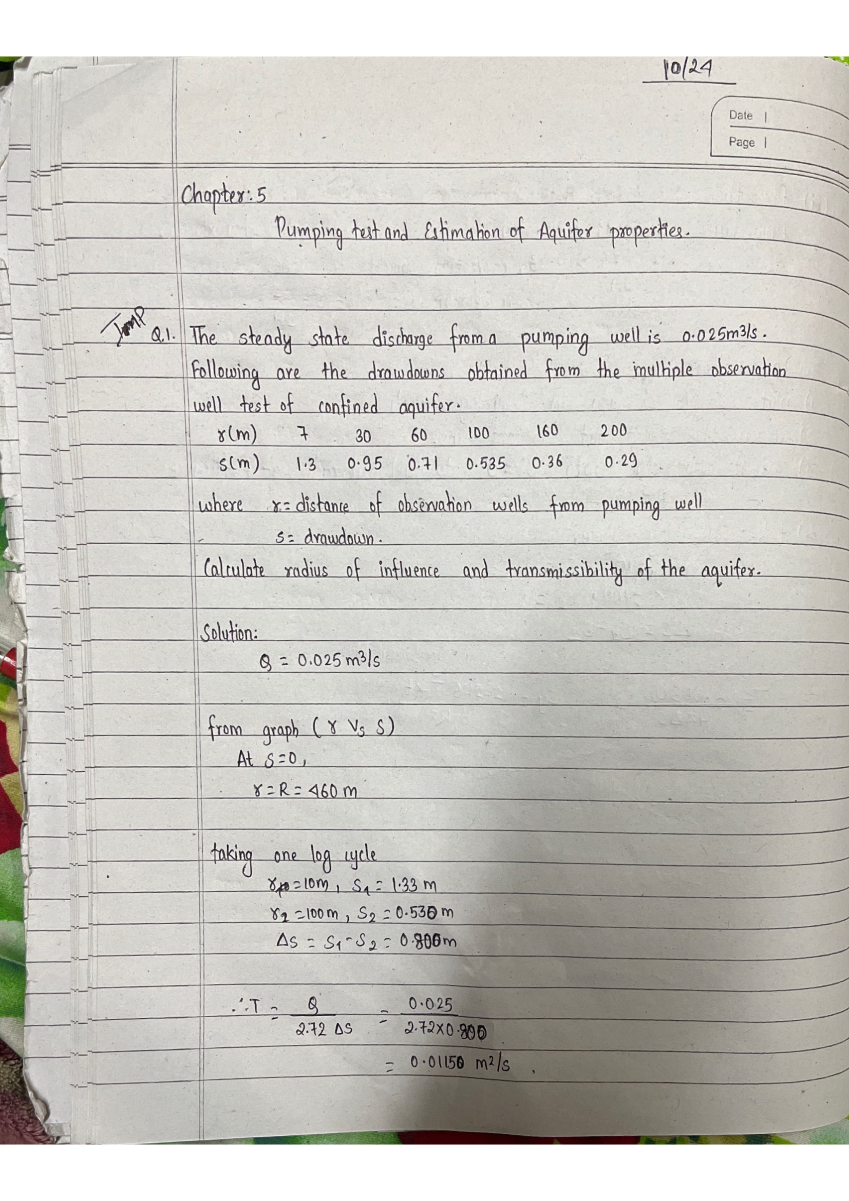
Numerical 1 – Distance-Drawdown (Confined)

Q. Q = 0.025 m³/s, confined aquifer:

r (m)73060100160200
s (m)1.30.950.710.5350.360.29
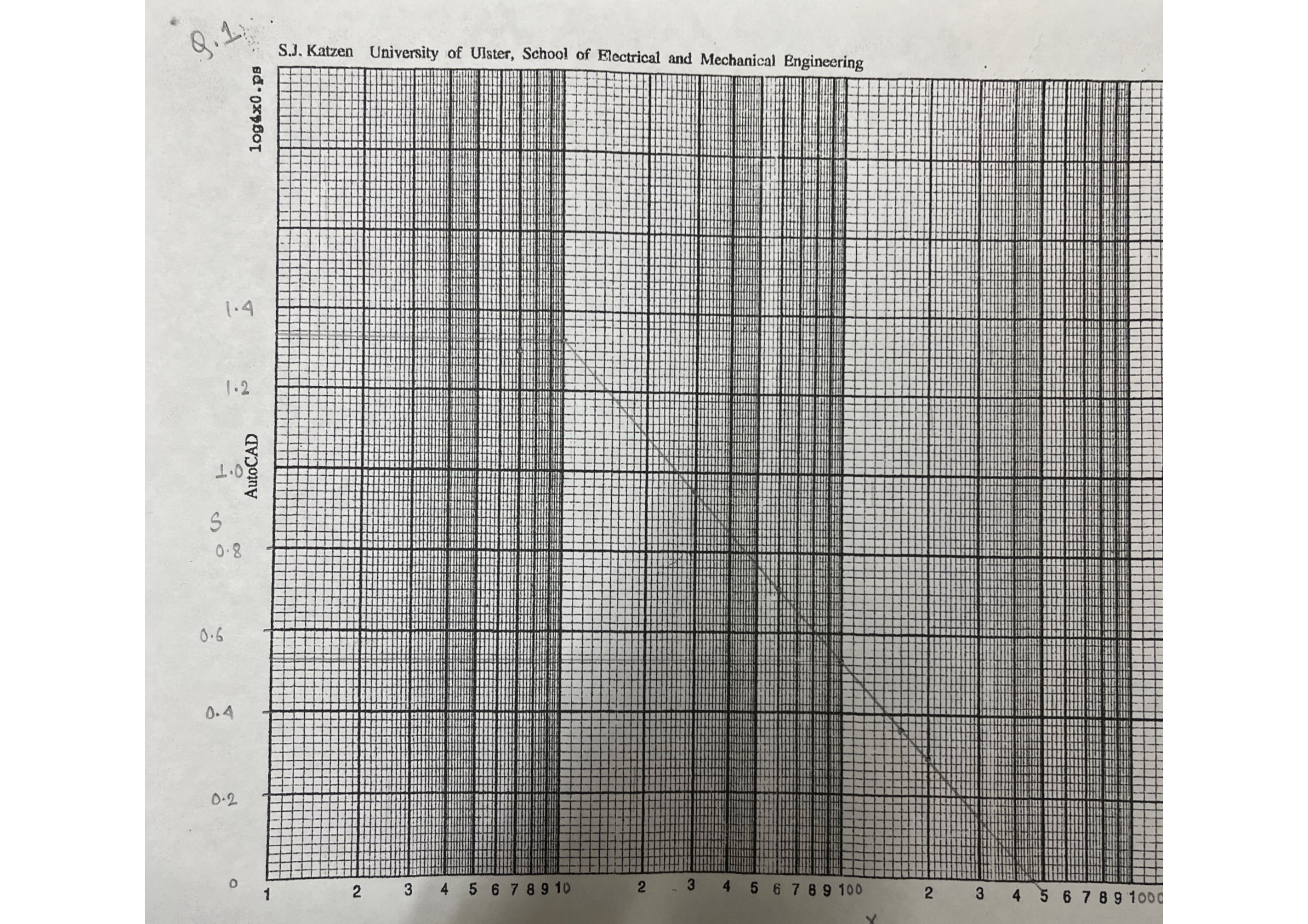
1 10 100 1000 r (m) → log scale 0 0.5 1.0 1.5 s (m) 7 30 60 100 160 200 R₀≈460 Δs = 0.80
Fig: Semi-log r vs s plot — distance-drawdown method

Solution:

Step 1 — Plot r (log scale) vs s (linear) on semi-log paper.

Step 2 — Draw best-fit straight line. Extend to s=0 to get R0 ≈ 460 m.

Step 3 — Read Δs for 1 log cycle (r=10 to r=100): Δs = 1.33 − 0.530 = 0.800 m

Step 4 — Compute T:

\[ T = \frac{Q}{2.72\,\Delta s} = \frac{0.025}{2.72 \times 0.800} = \boxed{0.0115\;\text{m}^2\text{/s}} \]

Page 53

Page 53
Transcription

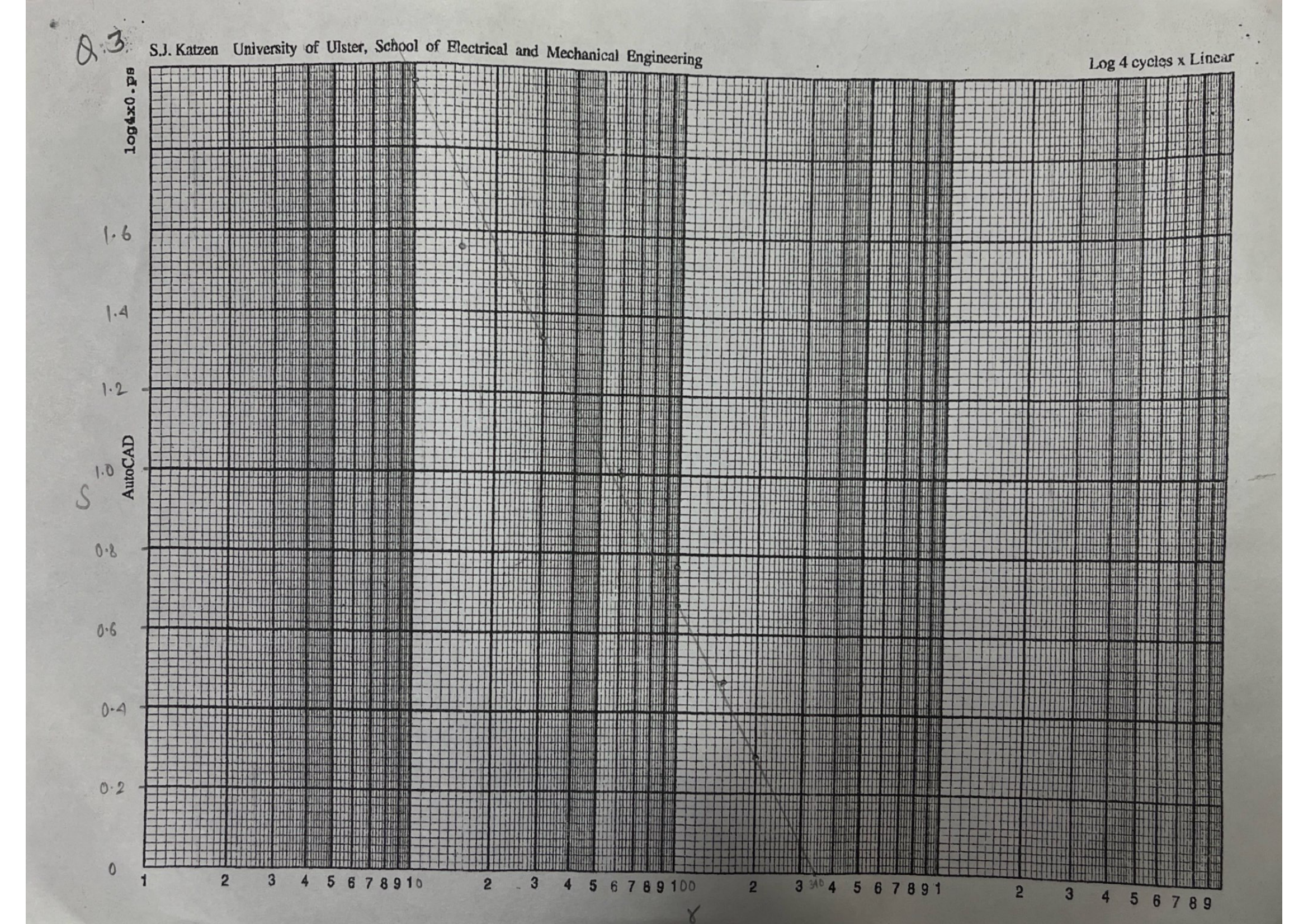
[Semi-log graph paper — Q1 Distance-Drawdown Plot]

  • x-axis (log): r (m), 4 cycles 1–1000
  • y-axis (linear): s (m), 0–1.5
  • 6 data points plotted, best-fit line
  • Extrapolated to s=0 at r ≈ 460m
  • 1 log cycle: r=10 (s=1.33) to r=100 (s=0.53), Δs=0.80

Page 54

Page 54
Transcription

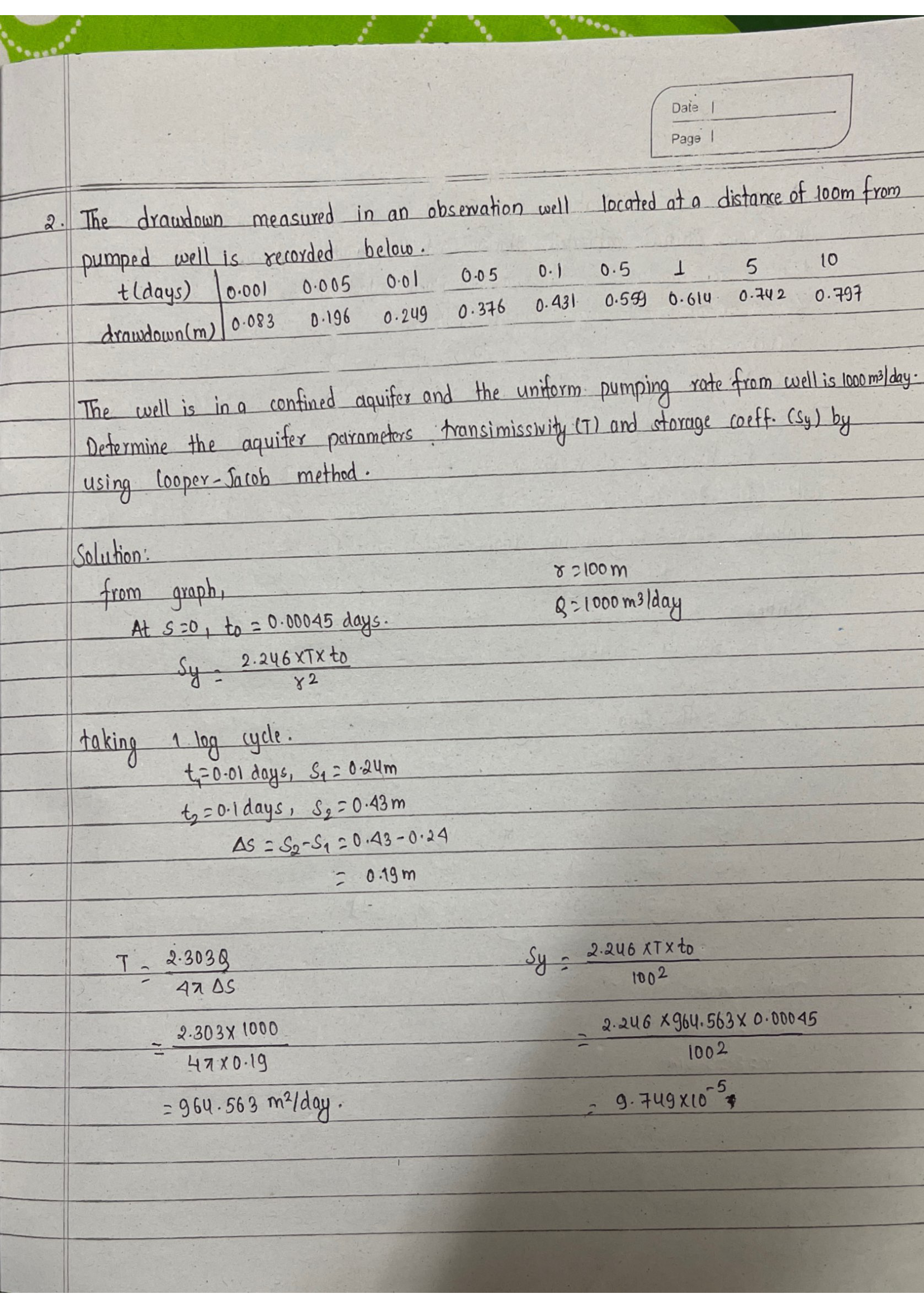
Numerical 2 – Time-Drawdown (Cooper-Jacob, Confined)

Q. r = 100 m, Q = 1000 m³/day:

t (days)0.0010.0050.010.050.10.51510
s (m)0.0830.1960.2490.3460.4310.5390.6140.7420.797

Solution:

Step 1 — Plot t (log scale) vs s (linear) on semi-log paper.

Step 2 — Draw best-fit straight line through the data points.

Step 3 — Extend line to s=0 to find t0 = 0.00045 days.

Step 4 — Read Δs per log cycle: Δs = 0.43 − 0.24 = 0.19 m

Step 5 — Compute T:

\[ T = \frac{2.303 \times Q}{4\pi \times \Delta s} = \frac{2.303 \times 1000}{4\pi \times 0.19} = \frac{2303}{2.388} = \boxed{964.6\;\text{m}^2\text{/day}} \]

Step 6 — Compute S:

\[ S = \frac{2.246\,T\,t_0}{r^2} = \frac{2.246 \times 964.6 \times 0.00045}{100^2} = \frac{0.975}{10000} = \boxed{9.75 \times 10^{-5}} \]

Check: S in range 10−5 to 10−3 for confined aquifer. ✓
Page 55

Page 55
Transcription

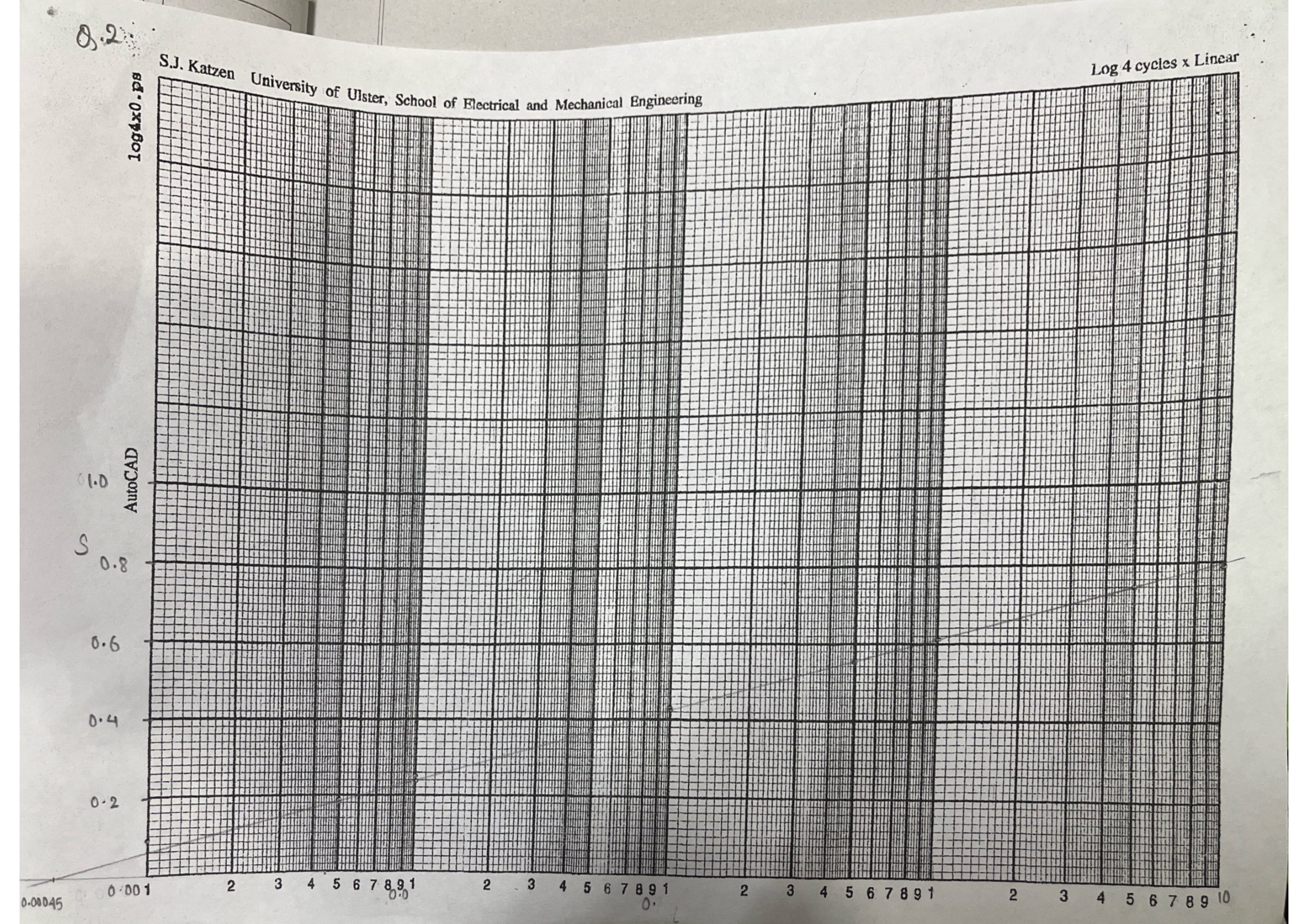
[Semi-log graph paper — Q2 Time-Drawdown Plot]

  • x-axis (log): t (days), 4 cycles
  • y-axis (linear): s (m), 0–0.8
  • Best-fit line extrapolated to s=0 at t0 ≈ 0.00045 days
  • Δs per log cycle ≈ 0.19 m

Page 56

Page 56
Transcription

Numerical 3 – Unconfined, Distance-Drawdown (with correction)

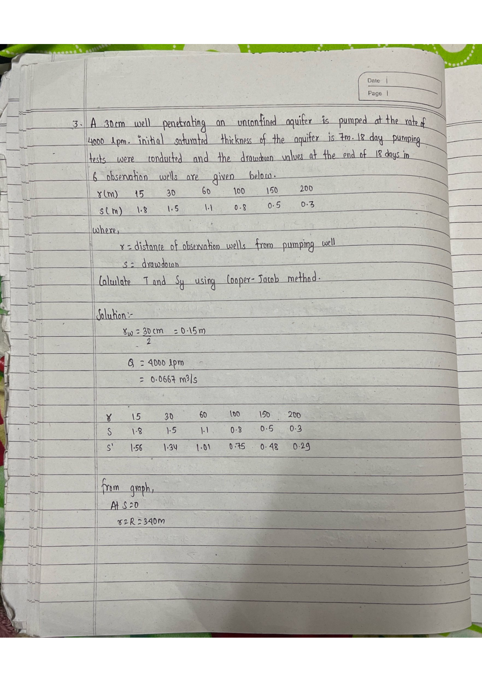
Q. Q = 4000 m³/day, H = 45 m. Observation wells:

r (m)1520406080100150
s (m)1.81.51.00.80.50.30.1
s′ (m)1.7641.4750.9890.7930.4970.2990.0999

Step 1 — Apply Jacob correction: s′ = s − s²/(2H), where H = 45 m

Sample calculation for r=15: s′ = 1.8 − 1.8²/(2×45) = 1.8 − 3.24/90 = 1.8 − 0.036 = 1.764

Correction is small here because s/H < 5%, but becomes significant for larger drawdowns.

Page 57

Page 57
Transcription

From graph (s′ vs r, semi-log):

Step 2 — Plot corrected s′ vs r on semi-log paper.

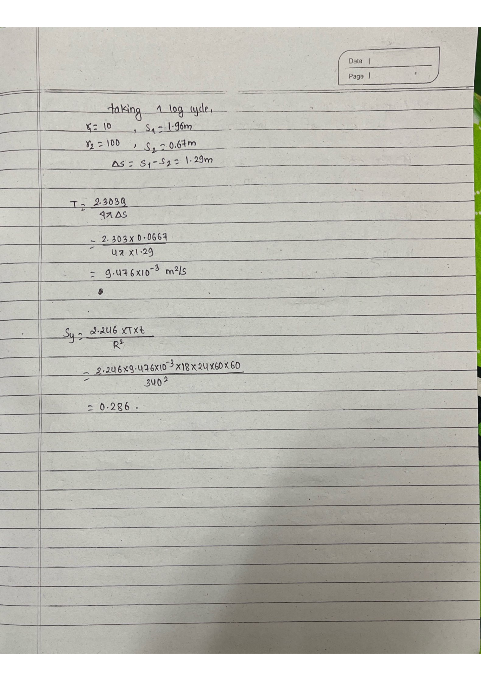
Step 3 — Read R0 = 210 m (where line meets s′=0), Δs′ = 0.64 m per log cycle.

Step 4 — Compute T:

\[ T = \frac{2.303 \times Q}{2\pi \times \Delta s'} = \frac{2.303 \times 4000}{2\pi \times 0.64} = \frac{9212}{4.021} = \boxed{2290.6\;\text{m}^2\text{/day}} \]

Step 5 — Compute K:

K = T/H = 2290.6/45 = 50.9 m/day

Step 6 — Sy (requires t0 from time data):

\( S_y = \frac{2.25\,T\,t_0}{r_0^2} \)

Page 58

Page 58
Transcription

[Semi-log graph paper — Q3 Corrected Drawdown Plot]

  • x-axis (log): r (m), 4 cycles 1–10000
  • y-axis (linear): s′ (m), 0–2.0
  • 7 data points, best-fit line
  • Extrapolated to s′=0 at r0 ≈ 210 m
  • Δs′ per log cycle ≈ 0.64 m