← All Chapters
Summary Note 4 / 7

Chapter 4 – Well Hydraulics (Formulae & Numericals)

GWE Handwritten Notes

Page 33

Page 33
Transcription

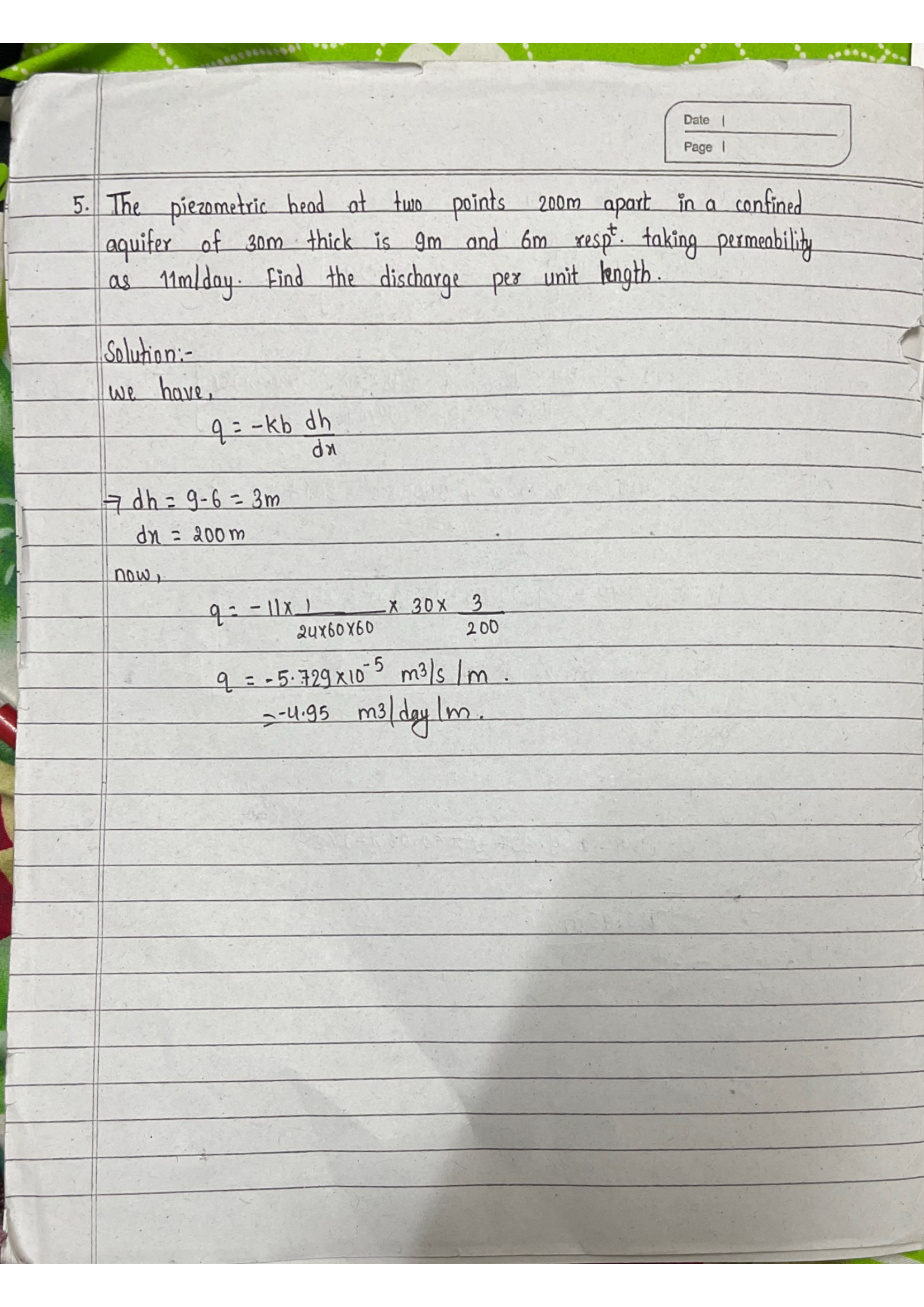
Numerical 5 – Confined Aquifer Discharge (Constant Thickness)

Q. Two obs. wells 200 m apart, confined aquifer b = 30 m, heads 9 m and 6 m. K = 11 m/day. Find q.

[Diagram: Confined aquifer cross-section, two wells, b=30m, h1=9m, h2=6m, L=200m]

Confining Layer Confined Aquifer (b = 30 m) Well 1 h₁=9m Well 2 h₂=6m Piezometric Surface L = 200 m q → b
Fig: Confined aquifer with two observation wells

Given: L = 200 m, b = 30 m, h1 = 9 m, h2 = 6 m, K = 11 m/day

Solution:

Step 1 — Hydraulic gradient: i = (h1 − h2)/L = (9 − 6)/200 = 0.015

Step 2 — Discharge per unit width (Darcy):

\[ q = K \cdot b \cdot i = 11 \times 30 \times 0.015 = \boxed{4.95\;\text{m}^2\text{/day/m}} \]

Step 3 — Convert to SI:

\[ q = \frac{4.95}{86400} = \boxed{5.729 \times 10^{-5}\;\text{m}^3\text{/s/m}} \]
Page 34

Page 34
Transcription

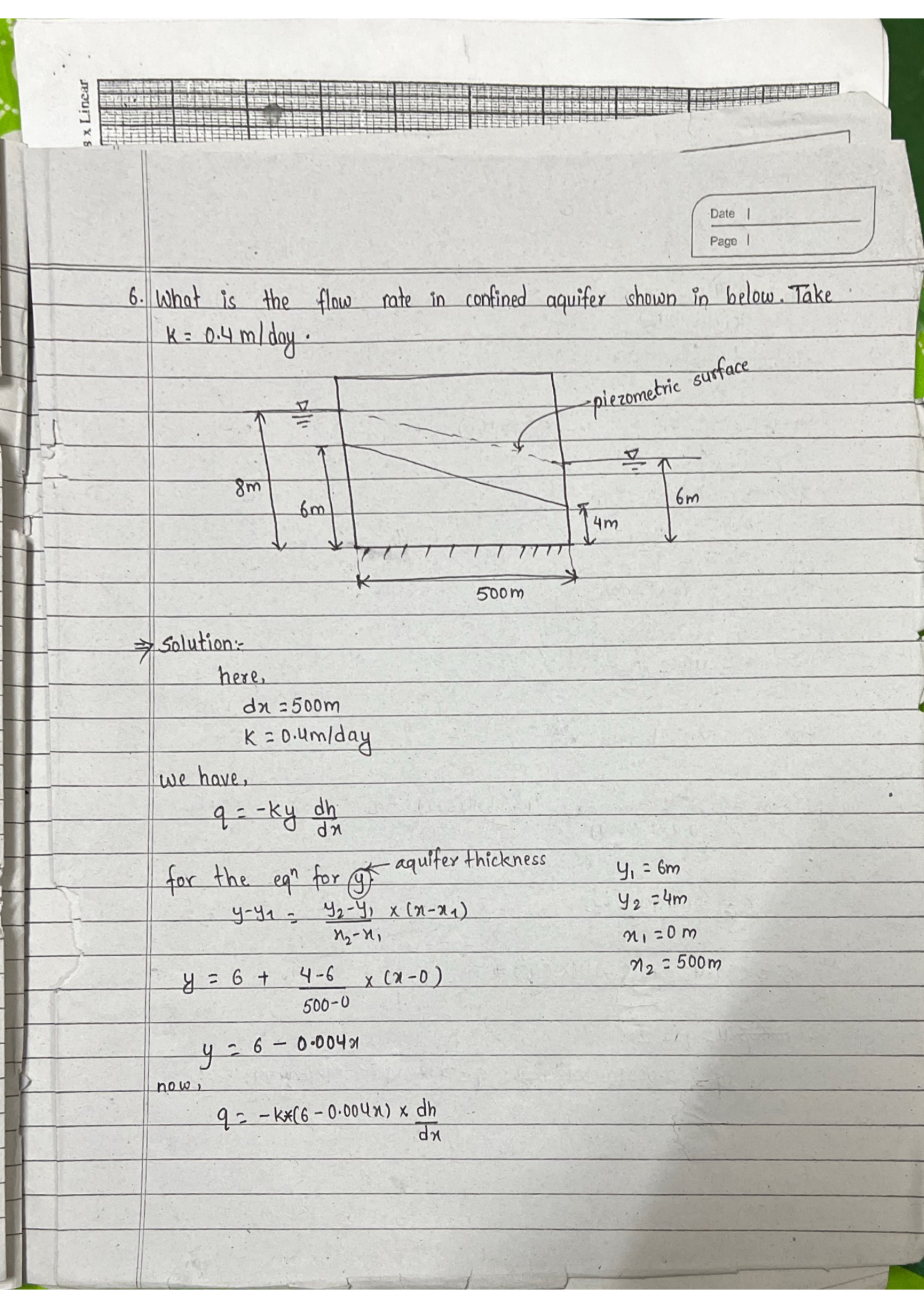
Numerical 6 – Confined Aquifer (Variable Thickness)

Q. K = 0.4 m/day. Left: h1=8m, y1=6m. Right: h2=6m, y2=4m. L=500m. q=?

[Diagram: Wedge-shaped confined aquifer, tapering from 6m to 4m over 500m]

Confined Aquifer (wedge-shaped) y₁=6m y₂=4m h₁=8m h₂=6m L = 500 m
Fig: Wedge-shaped confined aquifer with variable thickness

Solution:

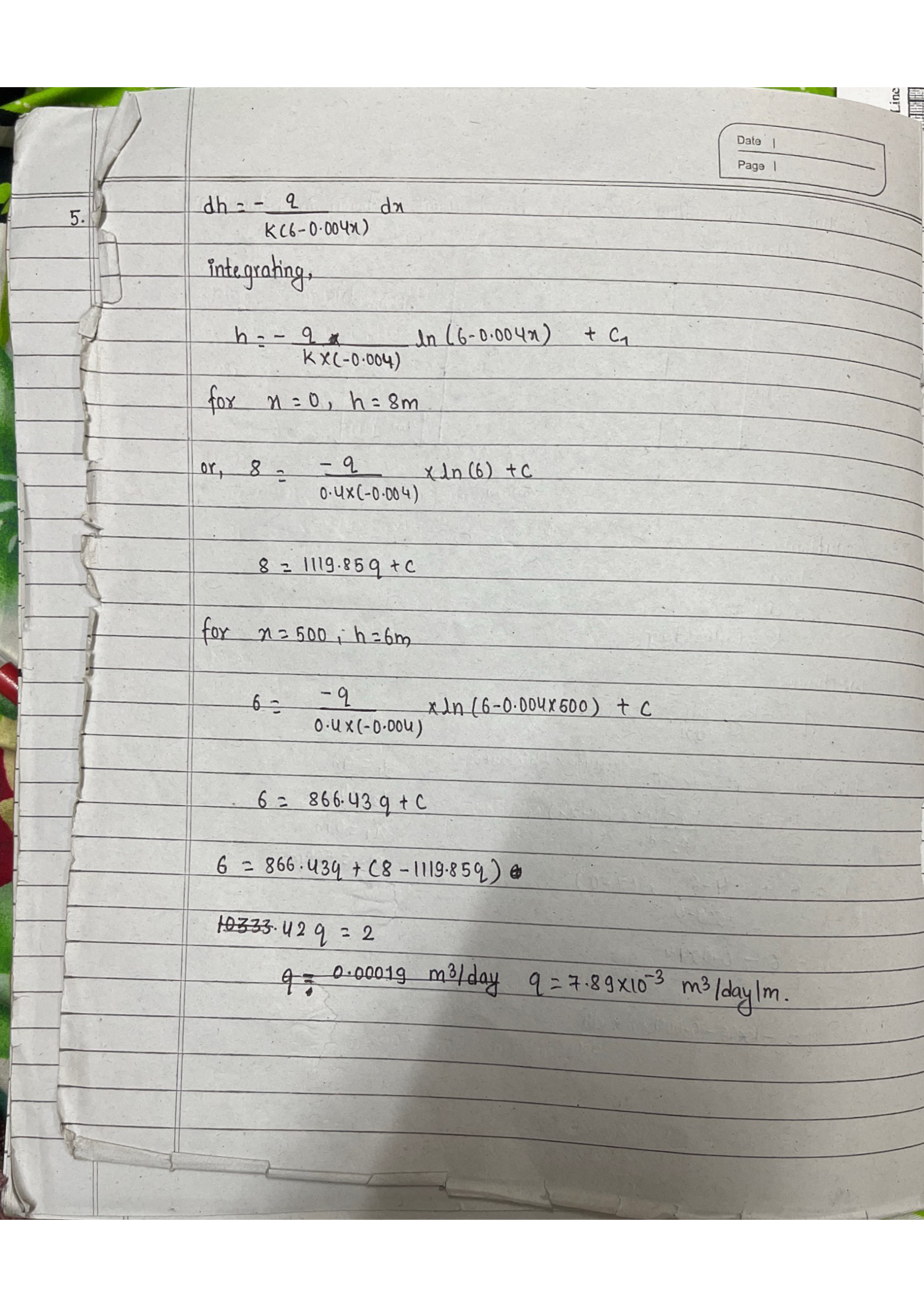
y(x) = 6 − 0.004x

\[ q = -K \cdot y(x) \cdot \frac{dh}{dx} \quad\Rightarrow\quad dh = \frac{-q}{K(6 - 0.004x)} dx \]

Integrating:

\[ h = \frac{q}{K \times 0.004} \ln(6 - 0.004x) + C \]

Page 35

Page 35
Transcription

(Continuing Numerical 6)

h = 625q · ln(6 − 0.004x) + C

B.C. 1: x=0, h=8: 8 = 625q × ln(6) + C = 1119.85q + C …(i)

B.C. 2: x=500, h=6: 6 = 625q × ln(4) + C = 866.41q + C …(ii)

Subtracting: 2 = 253.44q

\[ q = \frac{2}{253.44} = \boxed{7.89 \times 10^{-3} \text{ m}^2\text{/day/m}} \]

C = 8 − 1119.85 × 7.89×10−3 = −0.835

Piezometric surface: h(x) = 4.931 ln(6 − 0.004x) − 0.835

Page 36

Page 36
Transcription

Date: 09/15

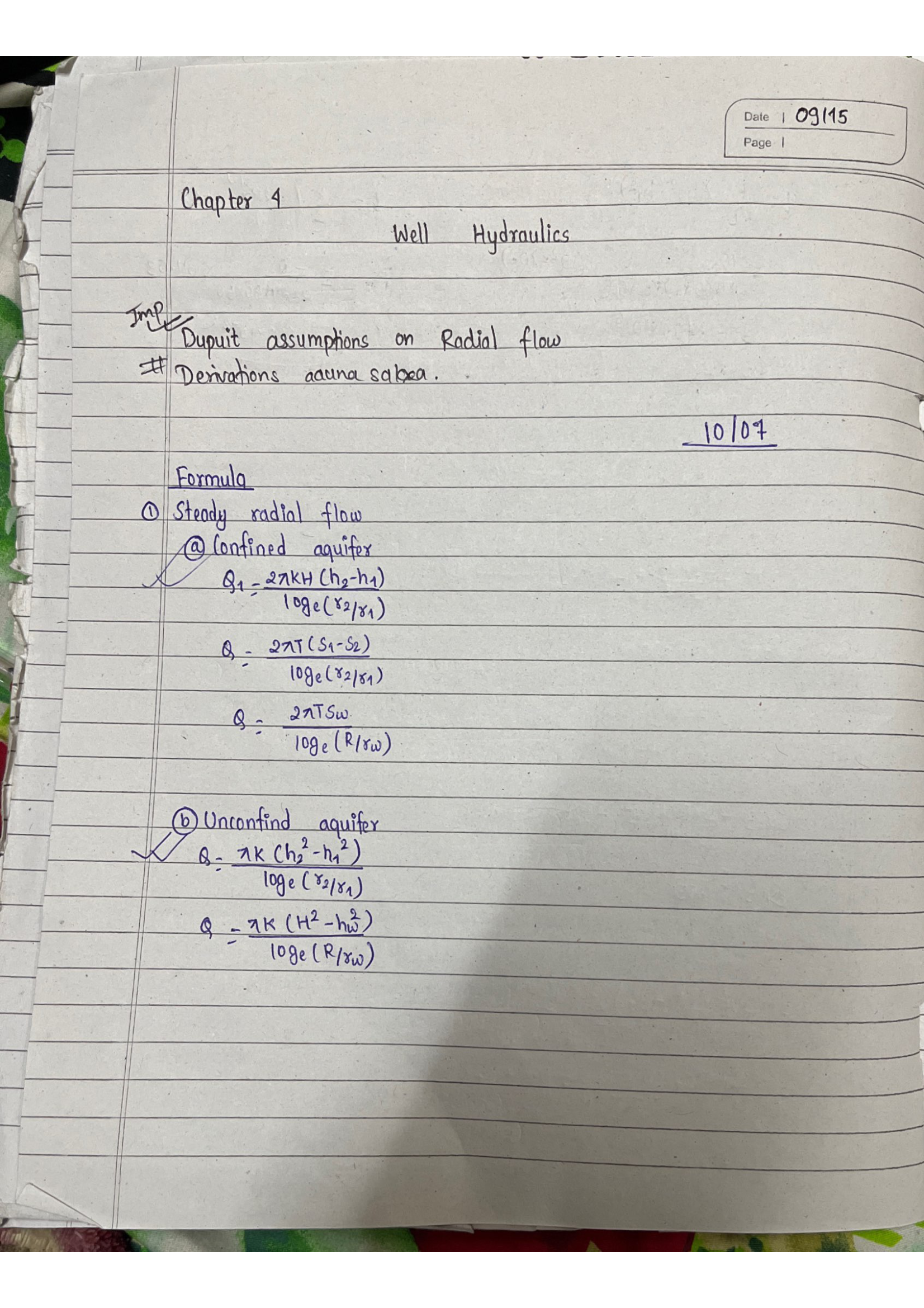
Chapter 4 – Well Hydraulics

Important: Dupuit assumptions on Radial flow. Derivations may be asked.

Ground Surface Confining Layer Q ↑ Static H s₂ s₁ Sᵤ r₁ r₂ R (radius of influence) b Confined Aquifer
Fig: Pumping well in confined aquifer — cone of depression in piezometric surface

① Steady Radial Flow

(a) Confined aquifer:

\[ Q = \frac{2\pi K b (h_2 - h_1)}{\ln(r_2/r_1)} = \frac{2\pi T (S_1 - S_2)}{\ln(r_2/r_1)} = \frac{2\pi T S_w}{\ln(R/r_w)} \]

(b) Unconfined aquifer:

\[ Q = \frac{\pi K (h_2^2 - h_1^2)}{\ln(r_2/r_1)} = \frac{\pi K (H^2 - h_w^2)}{\ln(R/r_w)} \]

Page 37

Page 37
Transcription

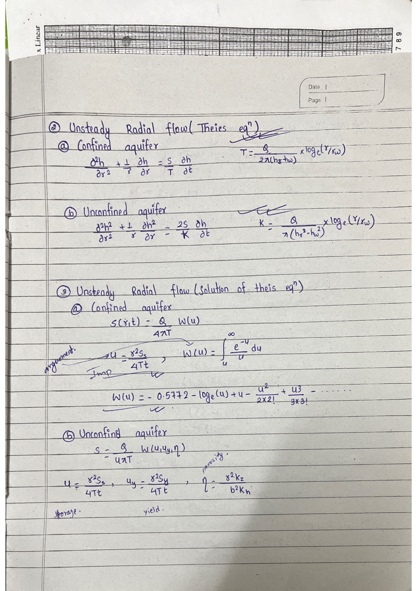
② Unsteady Radial Flow

(a) Confined:

\[ \frac{\partial^2 h}{\partial r^2} + \frac{1}{r}\frac{\partial h}{\partial r} = \frac{S}{T}\frac{\partial h}{\partial t} \]

(b) Unconfined:

\[ \frac{\partial^2 h^2}{\partial r^2} + \frac{1}{r}\frac{\partial h^2}{\partial r} = \frac{2S}{K}\frac{\partial h}{\partial t} \]

③ Theis Solution

\[ s(r,t) = \frac{Q}{4\pi T} W(u) \quad;\quad u = \frac{r^2 S}{4Tt} \]
\[ W(u) = -0.5772 - \ln(u) + u - \frac{u^2}{2 \cdot 2!} + \frac{u^3}{3 \cdot 3!} - \cdots \]

Page 38

Page 38
Transcription

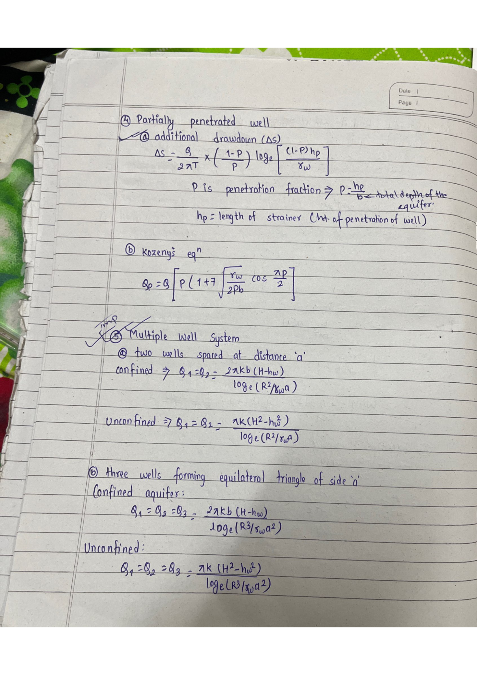
④ Partially Penetrating Well

[Diagram: Confined aquifer with partially penetrating well. Screen length hp < b. Flow lines bend toward shorter screen.]

P = hp/b (penetration fraction)

Additional drawdown:

\[ \Delta S_w = \frac{Q}{2\pi T} \cdot \frac{(1-P)}{P} \cdot \ln\frac{(1-P)h_p}{r_w} \]

Kozeny’s Equation:

\[ Q_p = Q\left[P\left(1 + 7\sqrt{\frac{r_w}{2Pb}}\right)\cos\frac{\pi P}{2}\right] \]

⑤ Multiple Well System

Two wells (distance a):

\[ Q = \frac{2\pi Kb(H-h_w)}{\ln(R^2/r_w a)} \]

Three wells (equilateral Δ, side a):

\[ Q = \frac{2\pi Kb(H-h_w)}{\ln(R^3/r_w a^2)} \]

Page 39

Page 39
Transcription

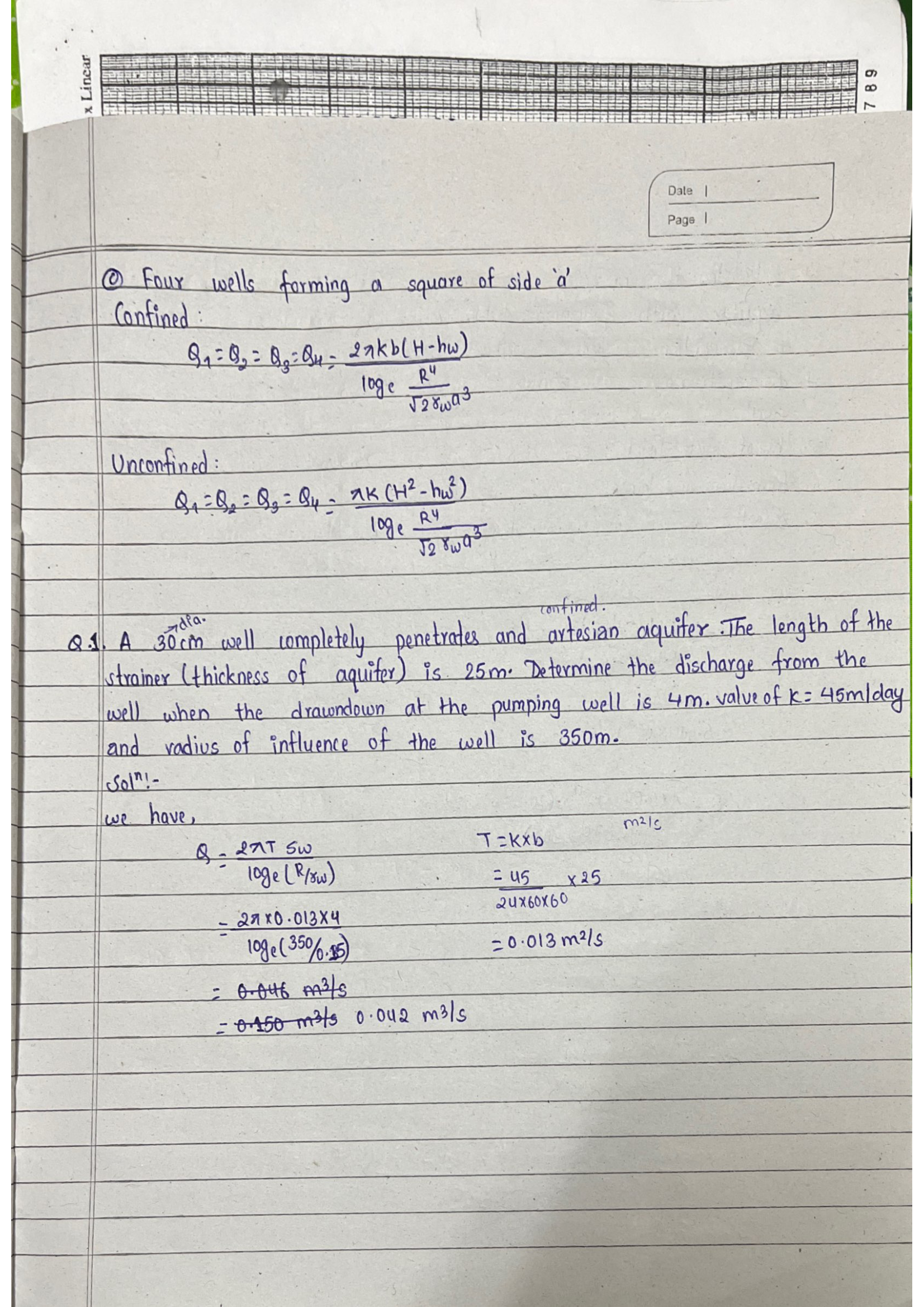
Four wells (square, side a):

\[ Q = \frac{2\pi Kb(H-h_w)}{\ln\frac{R^4}{\sqrt{2}\,r_w a^3}} \]

Numerical 1 – Confined Well (Find Q)

Q. 30cm dia. well, confined b=25m, Sw=4m, K=45m/day, R=350m.

Given: d=0.30m → rw=0.15m, b=25m, Sw=4m, K=45m/day, R=350m

Solution:

Step 1 — Compute transmissivity:

T = K × b = 45 × 25 = 1125 m²/day = 1125/86400 = 0.013 m²/s

Step 2 — Compute ln(R/rw):

ln(350/0.15) = ln(2333.3) = 7.754

Step 3 — Apply confined well formula:

\[ Q = \frac{2\pi T S_w}{\ln(R/r_w)} = \frac{2\pi \times 0.013 \times 4}{7.754} = \frac{0.3267}{7.754} = \boxed{0.042\;\text{m}^3\text{/s}} \]

Page 40

Page 40
Transcription

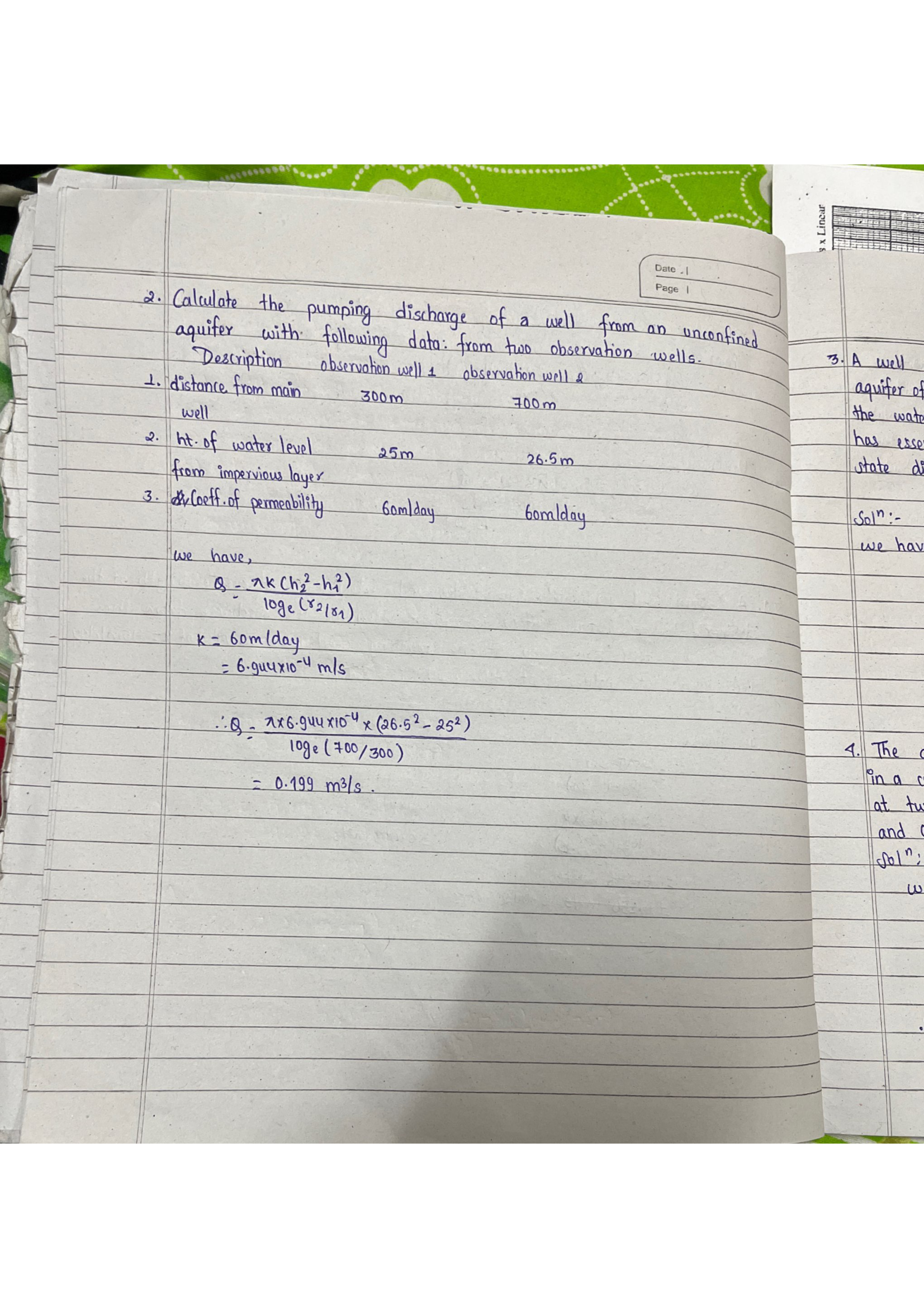
Numerical 2 – Unconfined, Two Obs. Wells (Find Q)

Q. r1=300m h1=25m, r2=700m h2=26.5m, K=60m/day.

Solution:

K = 60/86400 = 6.944×10⁻⁴ m/s

h2² − h1² = 702.25 − 625 = 77.25

ln(700/300) = 0.8473

\[ Q = \frac{\pi \times 6.944 \times 10^{-4} \times 77.25}{0.8473} = \boxed{0.199 \text{ m}^3\text{/s}} \]

Page 41

Page 41
Transcription

Date: 10/17

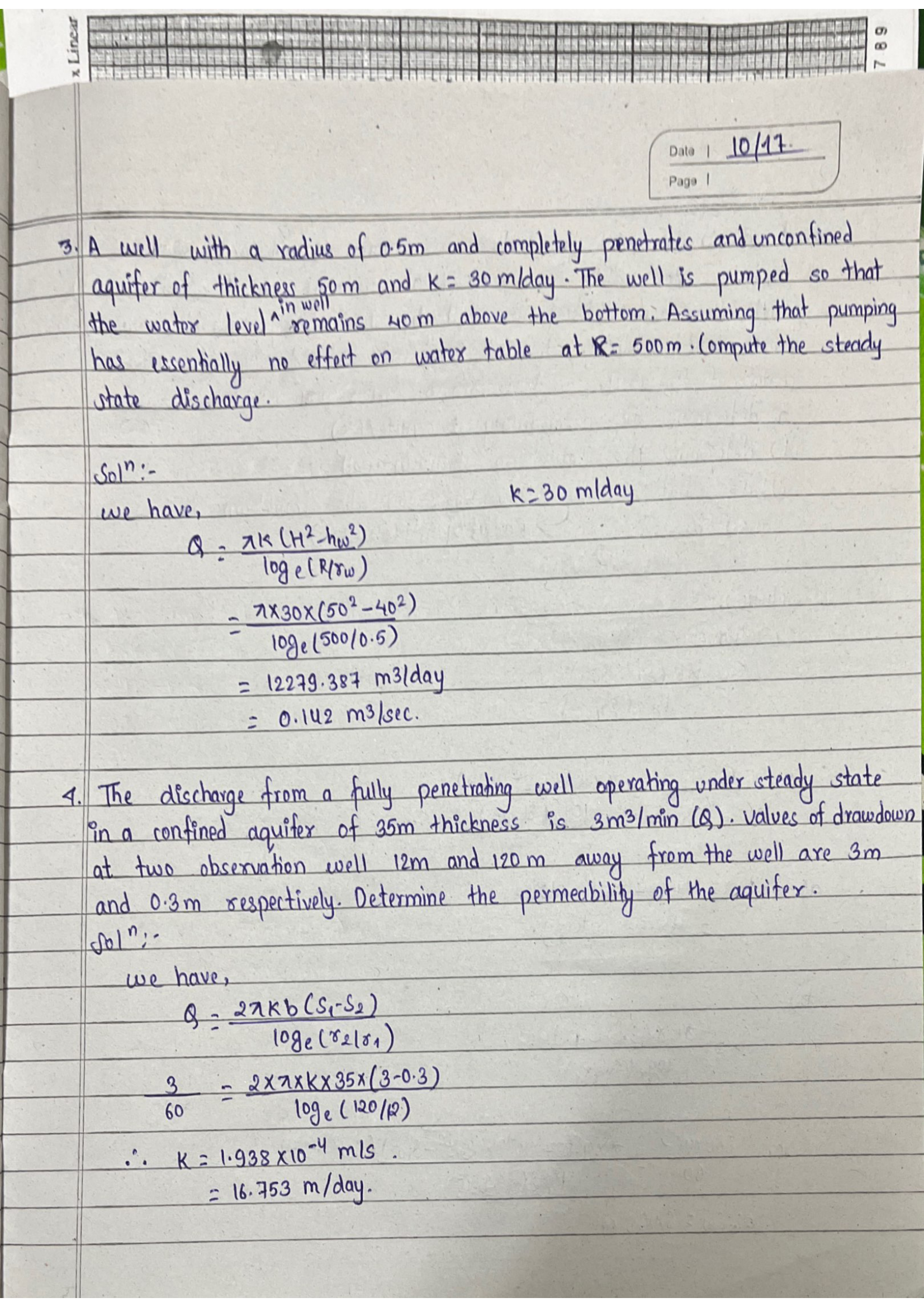
Numerical 3 – Unconfined, Steady State (Find Q)

Q. rw=0.5m, H=50m, K=30m/day, hw=40m, R=500m.

Solution:

H²−hw² = 2500−1600 = 900; ln(500/0.5) = 6.9078

\[ Q = \frac{\pi \times 30 \times 900}{6.9078} = 12279 \text{ m}^3\text{/day} = \boxed{0.142 \text{ m}^3\text{/s}} \]

Numerical 4 – Confined (Find K)

Q. Q=3 m³/min, b=35m, r1=12m S1=3m, r2=120m S2=0.3m.

Solution:

Q = 0.05 m³/s; ln(120/12) = 2.3026; S1−S2 = 2.7m

\[ T = \frac{0.05 \times 2.3026}{2\pi \times 2.7} = 6.786 \times 10^{-3} \text{ m}^2\text{/s} \]
\[ K = T/b = 1.938 \times 10^{-4} \text{ m/s} = \boxed{16.753 \text{ m/day}} \]

Page 42

Page 42
Transcription

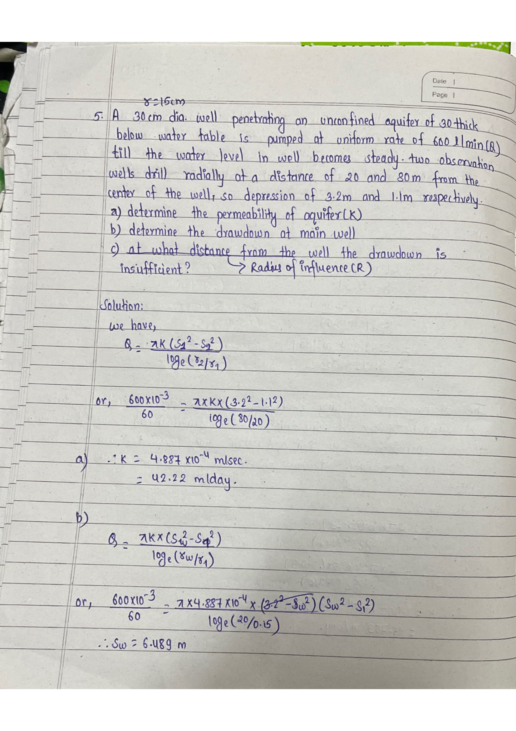
Numerical 5 – Unconfined (Find K, Sw, R)

Q. 30cm well, Q=600 l/min. r1=20m h1=1.1m, r2=80m h2=3.2m.

a) K:

h2²−h1² = 10.24−1.21 = 9.03; ln(4) = 1.3863

\[ K = \frac{0.6 \times 1.3863}{\pi \times 9.03} = 0.02933 \text{ m/min} = \boxed{42.22 \text{ m/day}} \]

b) Sw:

\[ \boxed{S_w = 6.489 \text{ m}} \]

Page 43

Page 43
Transcription

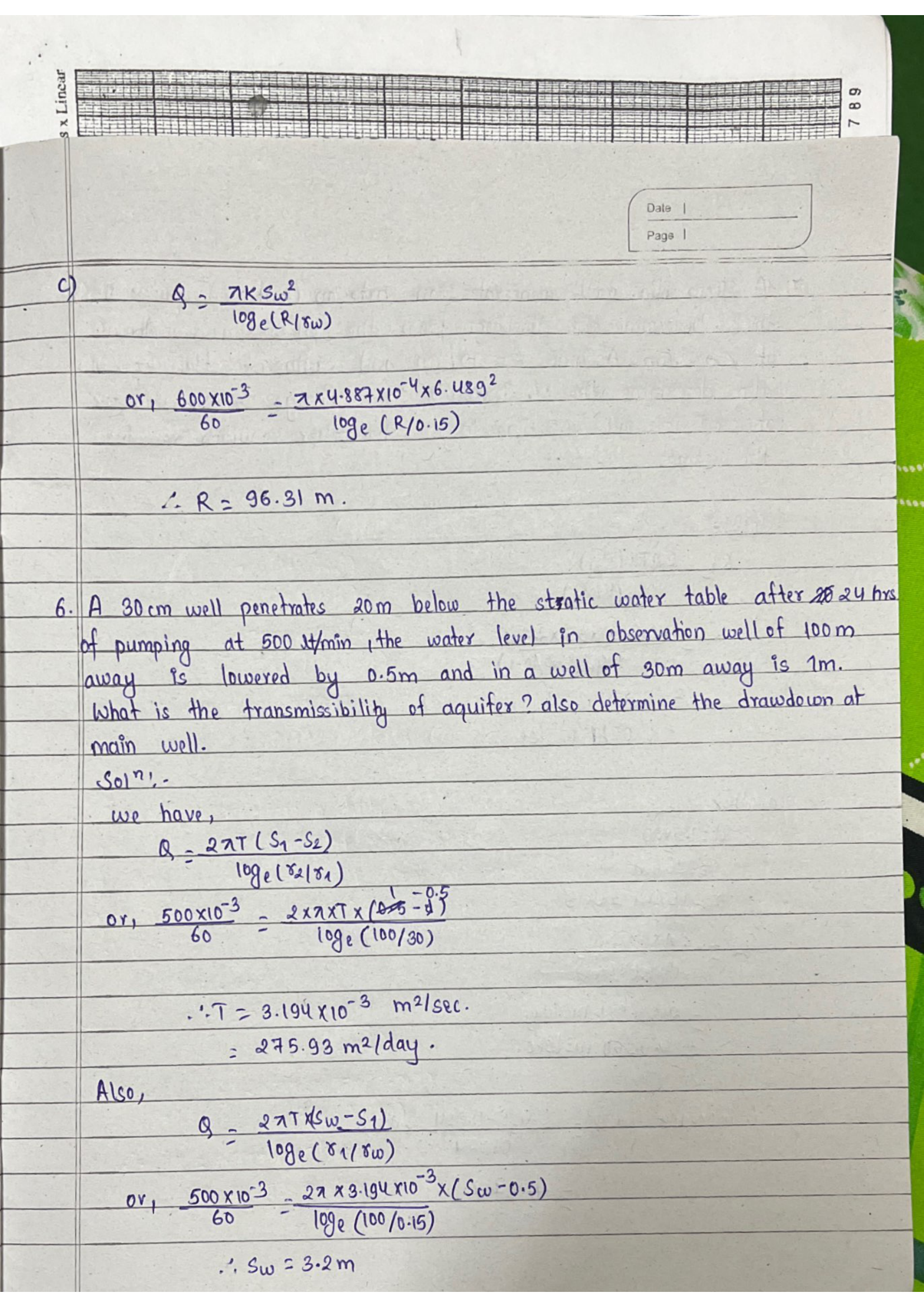
c) R:

\[ \boxed{R = 96.31 \text{ m}} \]

Numerical 6 – Confined (Find T, Sw)

Q. 30cm well, 20m below WT, Q=500 l/min. r1=30m S1=1m, r2=100m S2=0.5m.

Solution:

Q = 8.333×10⁻³ m³/s; ln(100/30) = 1.204; S1−S2=0.5

\[ T = \frac{8.333 \times 10^{-3} \times 1.204}{2\pi \times 0.5} = \boxed{3.194 \times 10^{-3} \text{ m}^2\text{/s} = 275.93 \text{ m}^2\text{/day}} \]

R = 30 × e2.408 = 333.3 m

\[ S_w = 0.4153 \times \ln(333.3/0.15) = 0.4153 \times 7.707 = \boxed{3.2 \text{ m}} \]

Page 44

Page 44
Transcription

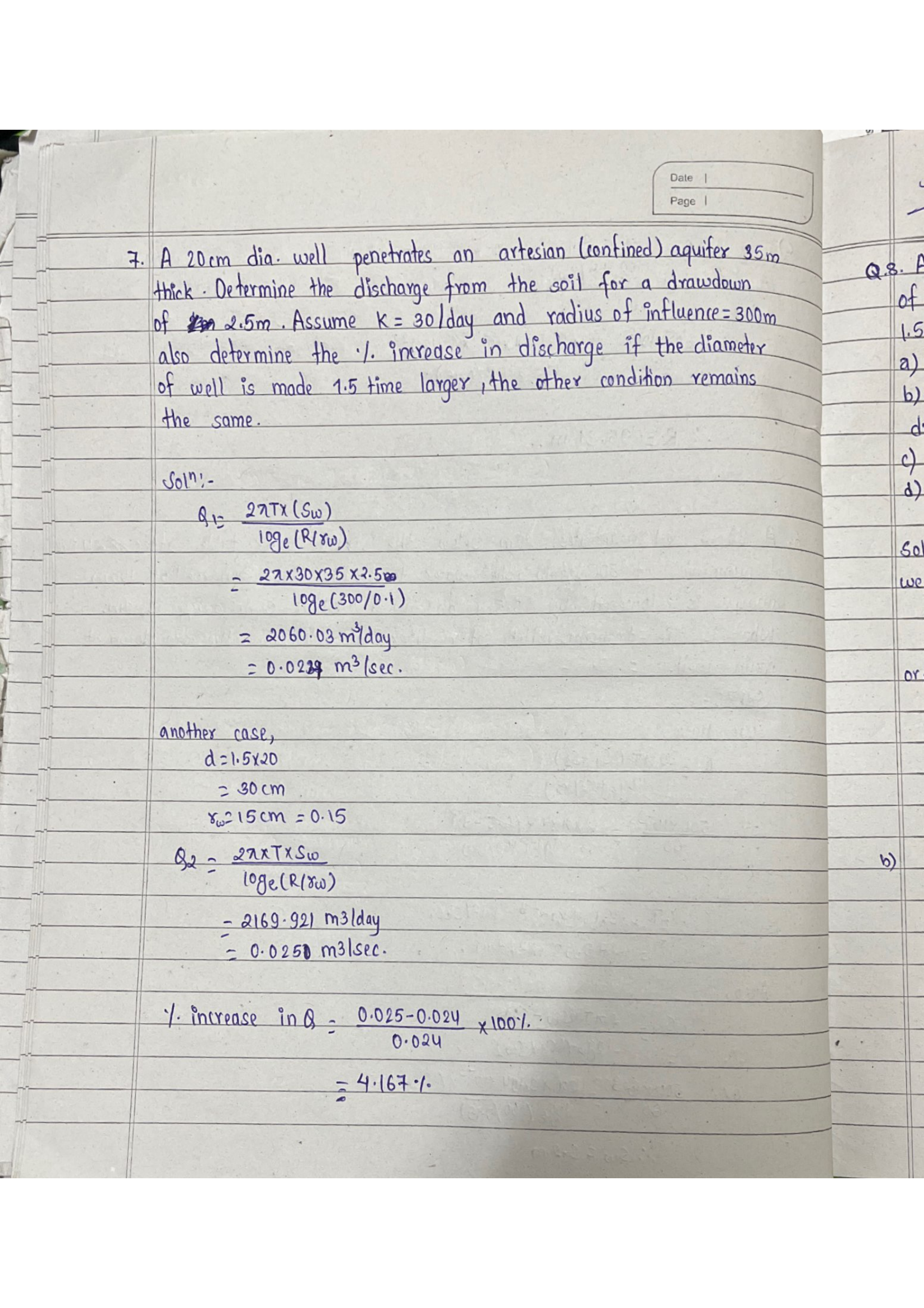
Numerical 7 – % Increase in Discharge

Q. 20cm well, confined b=35m, Sw=2.5m, K=30m/day, R=300m. Q=? Also % increase if d becomes 1.5× larger.

Solution:

T = 30×35 = 1050 m²/day

Case 1: d=20cm, rw=0.10m

\[ Q_1 = \frac{2\pi \times 1050 \times 2.5}{\ln(3000)} = \frac{16493}{8.006} = 2060 \text{ m}^3\text{/day} \]

Case 2: d=30cm, rw=0.15m

\[ Q_2 = \frac{16493}{\ln(2000)} = \frac{16493}{7.601} = 2170 \text{ m}^3\text{/day} \]
\[ \% \text{ increase} = \frac{2170-2060}{2060} \times 100 = \boxed{5.33\%} \]

Note: 50% increase in diameter gives only ~5% increase in Q due to logarithmic relationship.

Page 45

Page 45
Transcription

Date: 10/20

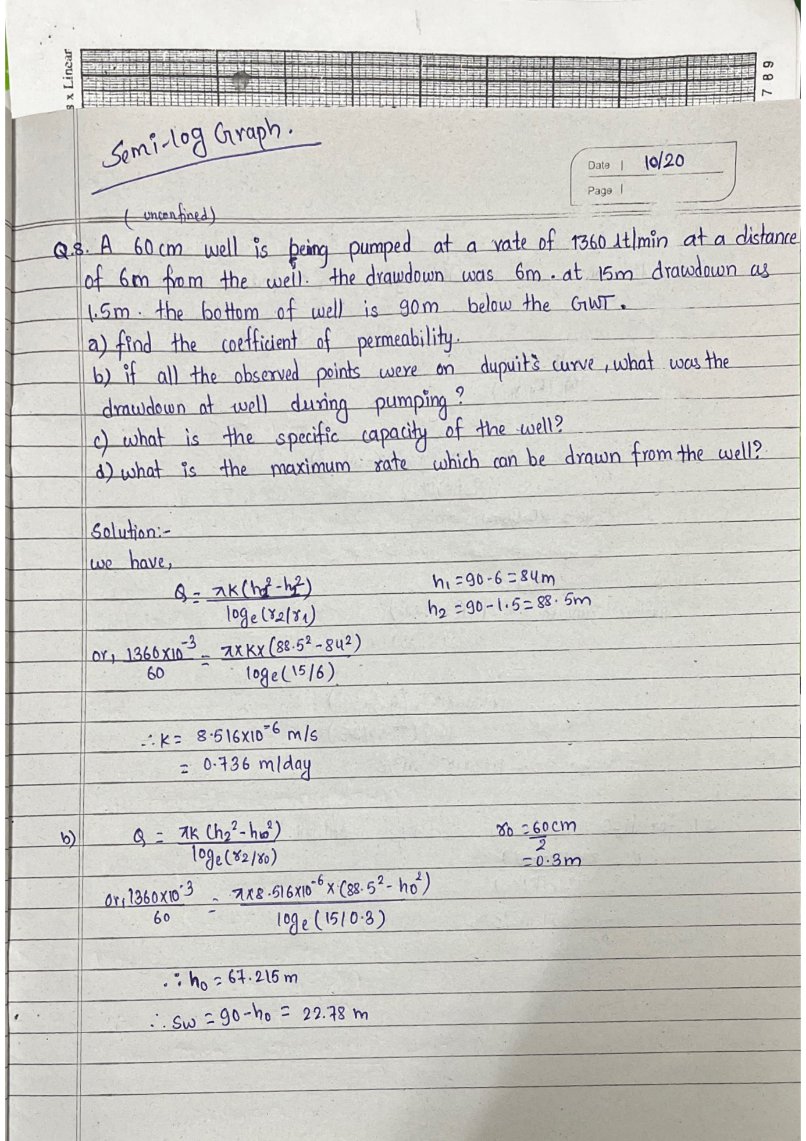
Numerical 8 – Unconfined (K, Sw, Specific Capacity, Qmax)

Q. 60cm dia. well, H=90m. At r=6m S=6m, at r=15m S=1.5m. Q=1360 l/min. Find K, Sw, specific capacity, max discharge.

Given: rw=0.3m, h1=84m, h2=88.5m, Q=0.02267 m³/s

a) K:

h2²−h1² = 7832.25−7056 = 776.25; ln(15/6)=0.9163

\[ K = \frac{0.02267 \times 0.9163}{\pi \times 776.25} = \boxed{8.516 \times 10^{-6} \text{ m/s} = 0.736 \text{ m/day}} \]

b) Sw:

Using Q = πK(h1²−h0²)/ln(r1/rw):

h0² = 7056 − 2539 = 4517 → h0 = 67.22m

\[ S_w = 90 - 67.22 = \boxed{22.78 \text{ m}} \]

Page 46

Page 46
Transcription

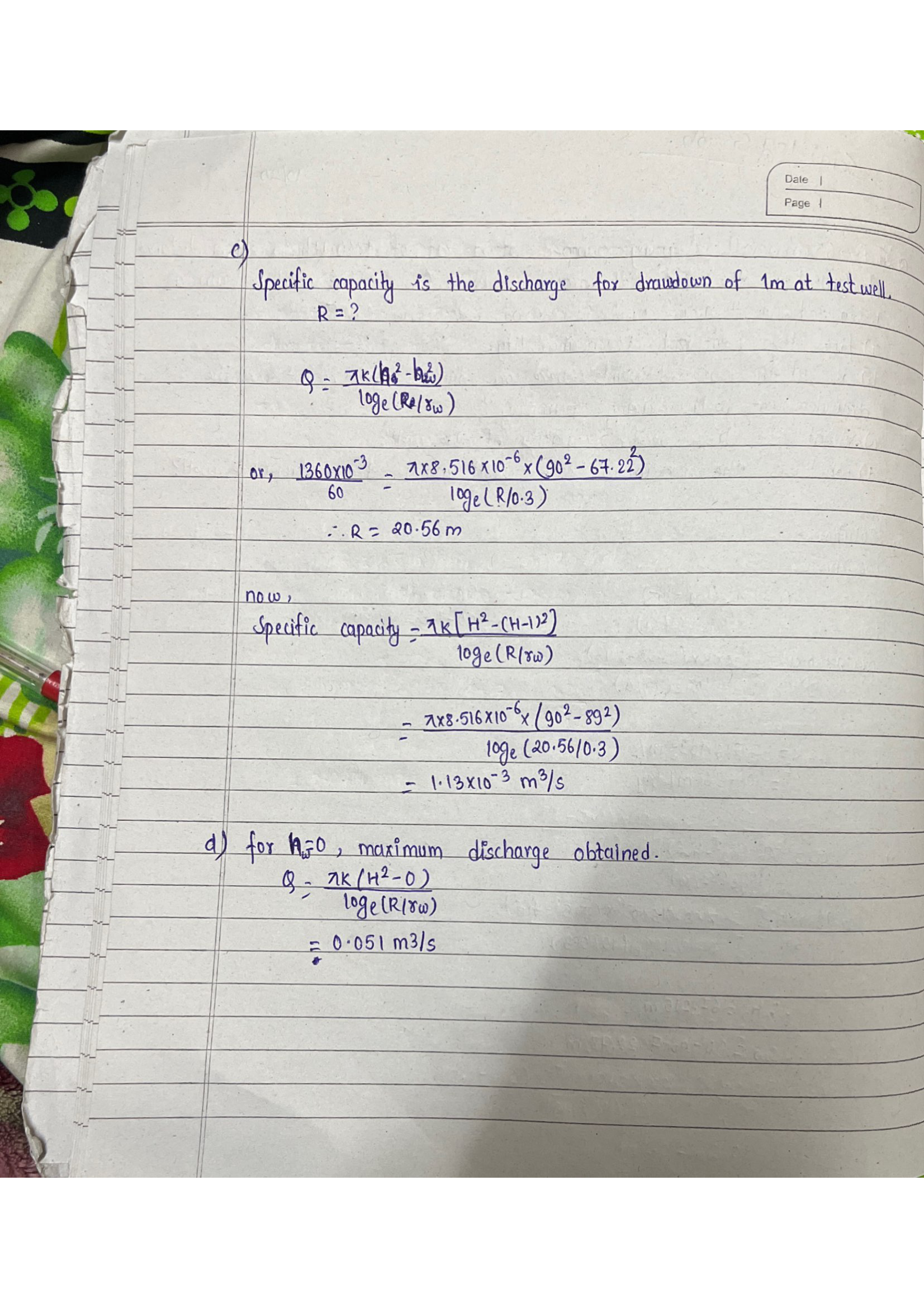
c) R & Specific Capacity:

ln(R/0.3) = 4.226 → R = 68.53×0.3 = 20.56 m

Specific capacity (Q for Sw=1m):

\[ Q_{sp} = \frac{\pi \times 8.516 \times 10^{-6} \times 179}{4.226} = \boxed{1.13 \times 10^{-3} \text{ m}^3\text{/s}} \]

d) Qmax (h0=0):

\[ Q_{max} = \frac{\pi K H^2}{\ln(R/r_w)} = \frac{2.675 \times 10^{-5} \times 8100}{4.226} = \boxed{0.051 \text{ m}^3\text{/s}} \]

Page 47

Page 47
Transcription

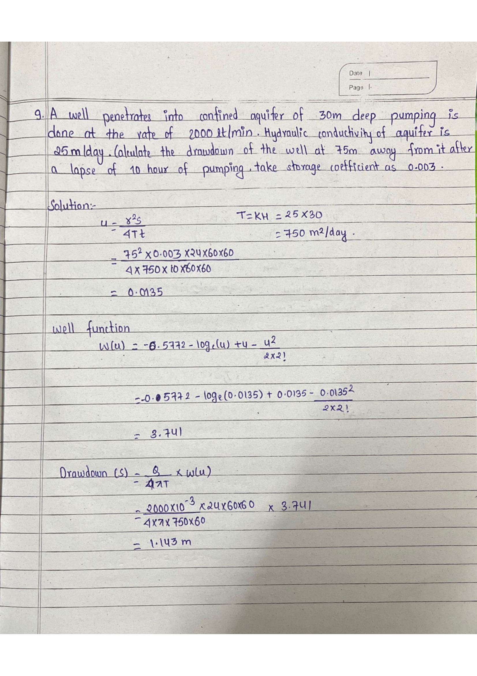
Numerical 9 – Theis / Well Function

Q. Confined b=30m, Q=2000 l/min, K=25m/day, r=75m, t=10hr, S=0.003. Drawdown=?

Given: b=30m, Q=2000 l/min, K=25 m/day, r=75m, t=10 hr, S=0.003

Solution:

Step 1 — Compute transmissivity:

T = K × b = 25 × 30 = 750 m²/day

Step 2 — Convert T to m²/s: T = 750/86400 = 8.68 × 10⁻³ m²/s

Step 3 — Convert t to days: t = 10/24 day

Step 4 — Compute u:

\[ u = \frac{r^2 S}{4Tt} = \frac{75^2 \times 0.003}{4 \times 750 \times (10/24)} = \frac{5625 \times 0.003}{1250} = \frac{16.875}{1250} = 0.0135 \]

Step 5 — Compute W(u) using the series:

\[ W(u) = -0.5772 - \ln(0.0135) + 0.0135 - \cdots \]

= −0.5772 + 4.3058 + 0.0135 = 3.741

Step 6 — Convert Q: Q = 2000/(60×1000) = 0.03333 m³/s

Step 7 — Compute drawdown:

\[ s = \frac{Q}{4\pi T} W(u) = \frac{0.03333}{4\pi \times 8.68 \times 10^{-3}} \times 3.741 = 0.3056 \times 3.741 = \boxed{1.143\;\text{m}} \]

Page 48

Page 48
Transcription

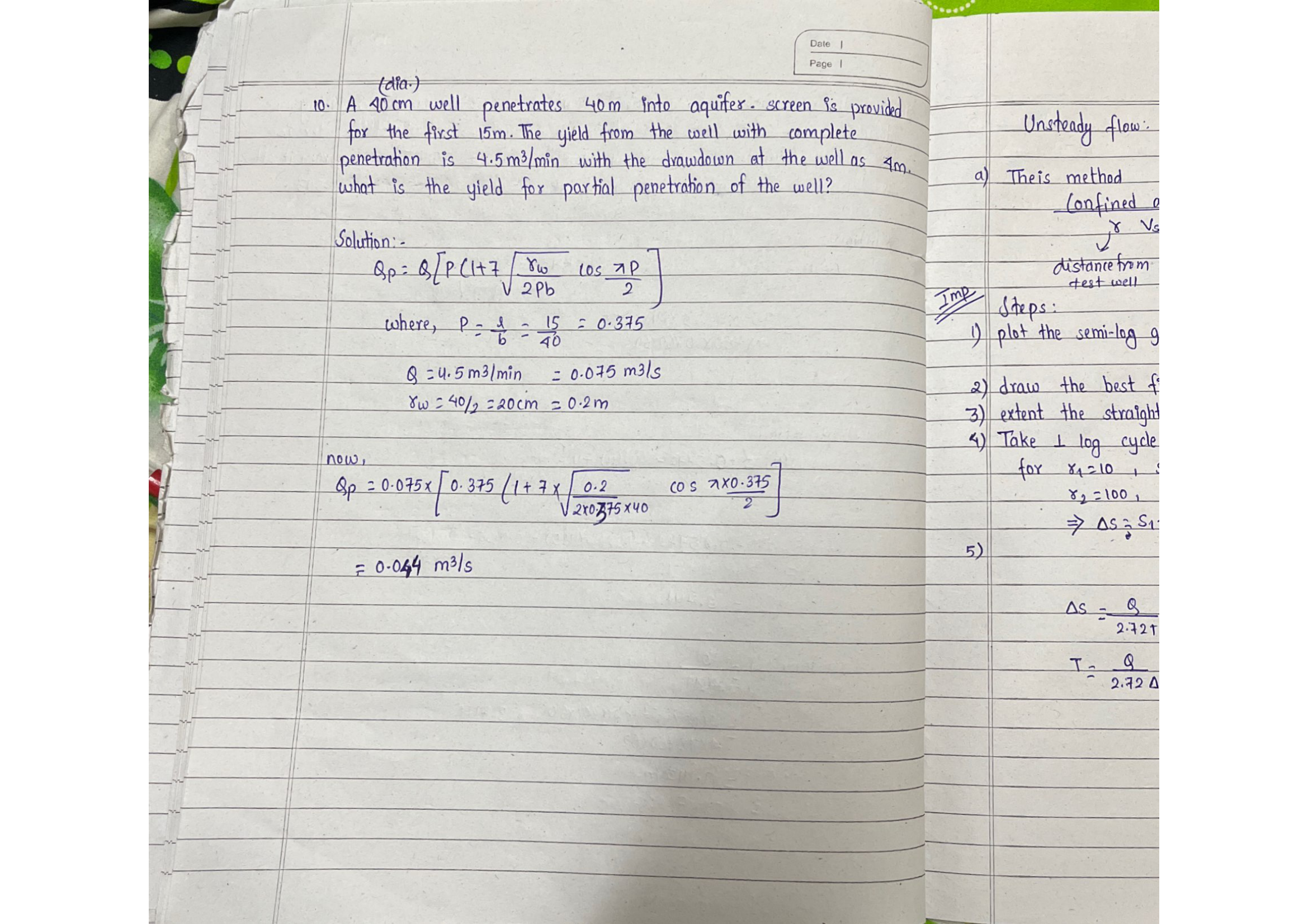
Numerical 10 – Partial Penetration (Kozeny)

Q. 40cm well, b=40m, screen 15m, full-pen Q=4.5 m³/min, Sw=4m. Partial-pen yield?

Solution:

P = 15/40 = 0.375; Q = 0.075 m³/s; rw=0.2m

\[ \frac{r_w}{2l_s} = \frac{0.2}{30} = 0.00667 \quad;\quad \sqrt{0.00667} = 0.0816 \]
\[ \frac{\pi P}{2} = 0.5890 \text{ rad} \quad;\quad \cos(0.5890) = 0.8315 \]
\[ \frac{Q_p}{Q} = 0.375 \times [1 + 7 \times 0.0816 \times 0.8315] = 0.375 \times 1.4752 = 0.553 \]
\[ Q_p = 0.075 \times 0.553 = \boxed{0.041 \text{ m}^3\text{/s}} \]

Margin Notes – Cooper–Jacob Method Steps:

  1. Plot semi-log graph: s (linear) vs r (log)
  2. Draw best-fit straight line
  3. Extend to s=0 → Radius of Influence (r0)
  4. Take 1 log cycle: Δs = s1 − s2
  5. \( T = \frac{Q}{2.72\,\Delta s} \)
  6. \( S = \frac{2.25\,T\,t}{r_0^2} \)