Chapter 3 – Flow Theory & Numericals

Page 21

Transcription

Date: 2081/09/12
Page |

Flow Net on anisotropic aquifer:

Water table contour map → draw contour lines → show flow direction.

Assume \( ds \approx dx \) (Dupuit assumption — flow is essentially horizontal, vertical velocity is negligible).

Flow in unconfined aquifer

Diagram: Cross-section of steady-state 1-D flow in a homogeneous, isotropic unconfined aquifer (Dupuit parabola).

Impervious base at bottom.
Left boundary: water height \( h_1 \) (higher head).
Right boundary: water height \( h_2 \) (lower head), \( h_1 > h_2 \).
Parabolic water table connecting \( h_1 \) to \( h_2 \).
Horizontal distance \( L \); at distance \( x \) from left: saturated thickness \( h \).
Discharge per unit width: \( q \).

Fig: Dupuit flow through unconfined aquifer — parabolic water table profile

Page 22

Transcription

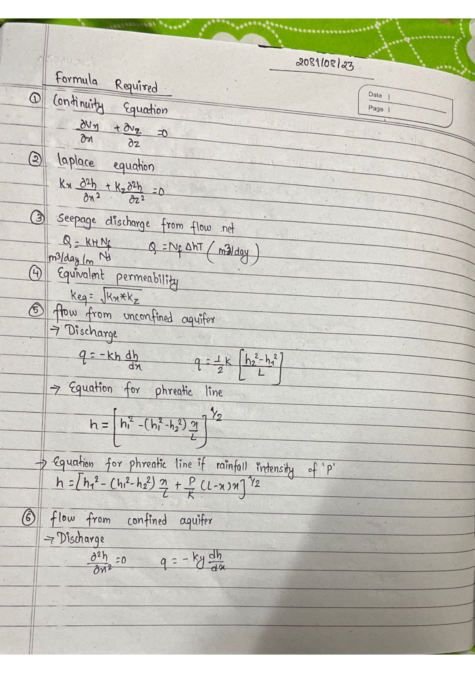
Formula Required

(Horizontal flow)

1. Continuity equation:

\[ \frac{\partial u}{\partial x} + \frac{\partial v}{\partial z} = 0 \]

2. Laplace equation:

\[ K_x \frac{\partial^2 h}{\partial x^2} + K_z \frac{\partial^2 h}{\partial z^2} = 0 \]

When \( K_x = K_z = K \): \( \frac{\partial^2 h}{\partial x^2} + \frac{\partial^2 h}{\partial z^2} = 0 \)

3. Seepage discharge from flow net:

\[ q = K H \frac{N_f}{N_d} \]

4. Equivalent Permeability:

\[ K_{eq} = \sqrt{K_x \cdot K_z} \]

5. Unconfined flow (Dupuit):

\[ q = \frac{K(h_1^2 - h_2^2)}{2L} \]

6. Phreatic line:

\[ h = \left[ h_1^2 - (h_1^2 - h_2^2)\frac{x}{L} \right]^{1/2} \]

With rainfall P:

\[ h = \left[ h_1^2 - (h_1^2 - h_2^2)\frac{x}{L} + \frac{P}{K}\, x(L - x) \right]^{1/2} \]

7. Confined flow:

\[ q = -K b \frac{dh}{dx} = \frac{K b (h_1 - h_2)}{L} \]

Page 23

Transcription

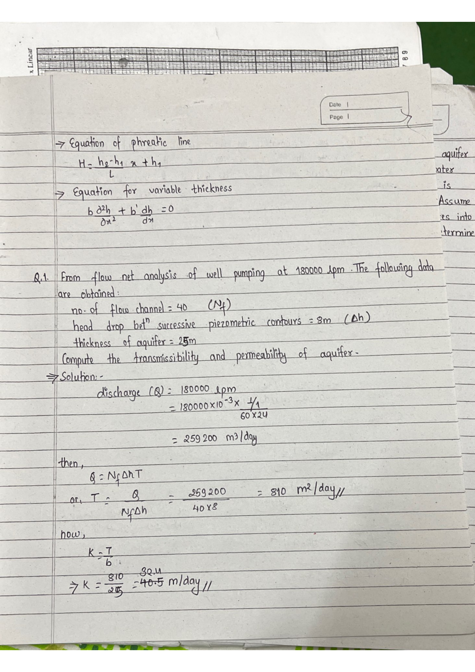
Phreatic line (confined): \( h^2 = h_1^2 - (h_1^2 - h_2^2) \frac{x}{L} \)

Variable thickness aquifer:

\[ b \frac{\partial^2 h}{\partial x^2} + b' \frac{\partial h}{\partial x} = 0 \]

Numerical – Flow Net Analysis

Q. From flow net analysis of well pumping at 180,000 lpm: N_f = 40, Δh = 8 m, b = 25 m. Compute T and K.

Given:

Q = 180,000 l/min
N_f = 40 (number of flow tubes)
Δh = 8 m (head loss per potential drop)
b = 25 m (aquifer thickness)

Solution:

Step 1 — Convert Q to m³/day:

\[ Q = 180{,}000 \;\text{l/min} \times \frac{10^{-3}\;\text{m}^3}{\text{l}} \times 60 \times 24 = 259{,}200\;\text{m}^3\text{/day} \]

Step 2 — Apply flow net relation \( Q = T \times N_f \times \Delta h \) to find T:

\[ T = \frac{Q}{N_f \times \Delta h} = \frac{259{,}200}{40 \times 8} = \boxed{810 \;\text{m}^2\text{/day}} \]

Step 3 — Compute K from transmissivity:

\[ K = \frac{T}{b} = \frac{810}{25} = \boxed{32.4 \;\text{m/day}} \]

Page 24

Transcription

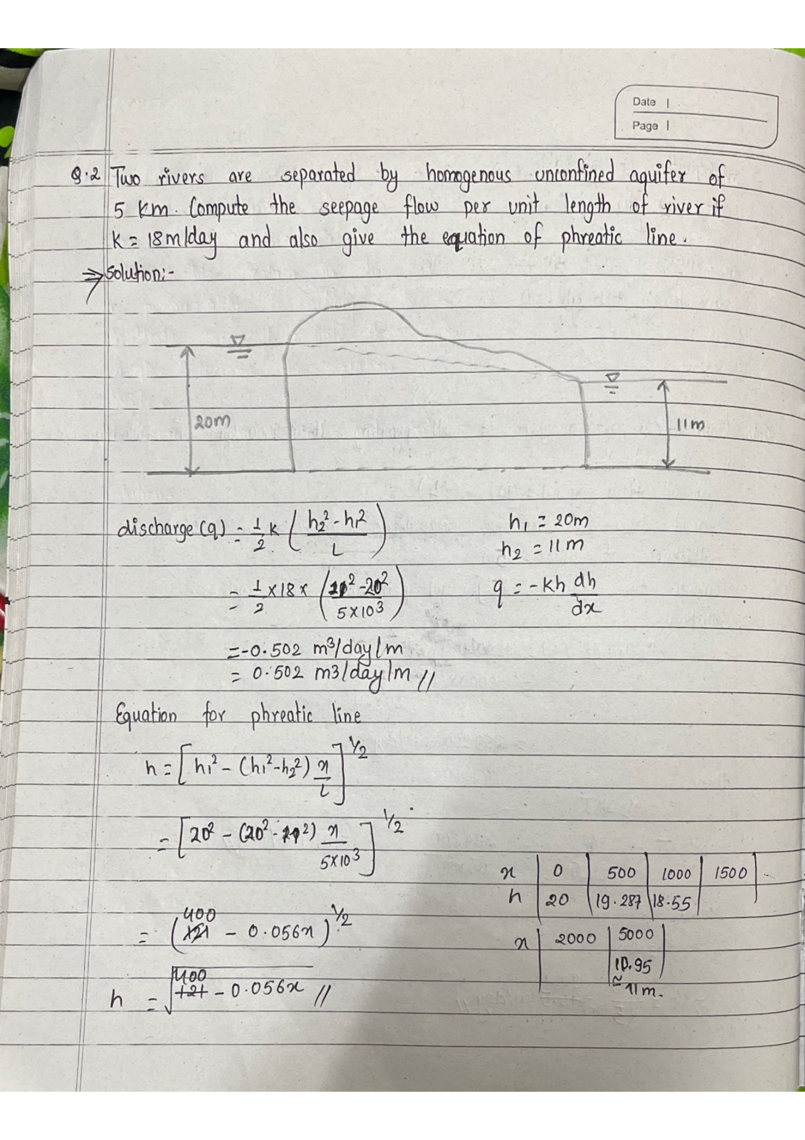
Numerical – Unconfined Flow Between Two Rivers

Q. Two rivers 5 km apart. K = 18 m/day, h₁ = 20 m, h₂ = 11 m. Seepage & phreatic line?

Fig: Steady Dupuit flow between two rivers

Given: L = 5000 m, K = 18 m/day, h₁ = 20 m, h₂ = 11 m

Solution:

Step 1 — Apply Dupuit formula for seepage per unit width:

\[ q = \frac{K(h_1^2 - h_2^2)}{2L} = \frac{18 \times (20^2 - 11^2)}{2 \times 5000} \]

Step 2 — Compute h₁² − h₂²:

= 400 − 121 = 279

Step 3 — Evaluate:

\[ q = \frac{18 \times 279}{10{,}000} = \boxed{0.502 \;\text{m}^2\text{/day/m}} \]

Step 4 — Phreatic line equation. Using \( h^2 = h_1^2 - (h_1^2 - h_2^2)\frac{x}{L} \):

\[ h = \sqrt{400 - \frac{279}{5000}\, x} = \sqrt{400 - 0.0558\, x} \]

Step 5 — Tabulate:

\( x \) (m)	0	500	1000	1500	2000	5000
\( h \) (m)	20	19.29	18.55	17.79	16.99	11

Page 25

Transcription

Date: 09/04
Page |

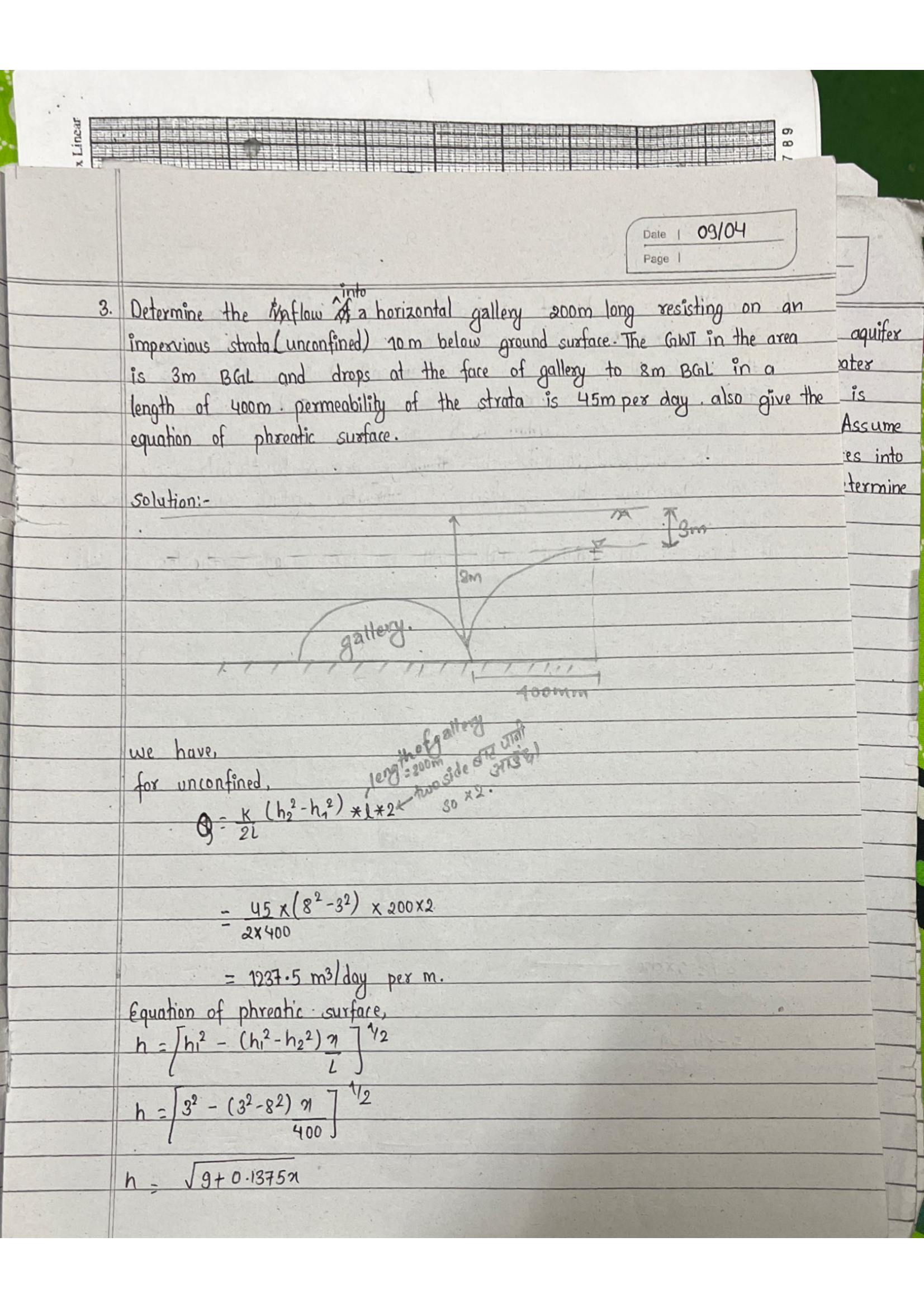
Numerical – Horizontal Gallery (Unconfined Aquifer)

Q. Gallery 200 m long on impervious stratum. h₂ = 8 m at 400 m, h₁ = 3 m at gallery face. K = 45 m/day. Find inflow and phreatic surface.

Fig: Gallery drawing water from both sides

Given: L_gallery = 200 m, L = 400 m, h₁ = 3 m, h₂ = 8 m, K = 45 m/day

Solution:

Step 1 — Seepage per unit width from one side (Dupuit):

\[ q = \frac{K(h_2^2 - h_1^2)}{2L} = \frac{45(64 - 9)}{800} = \frac{45 \times 55}{800} = 3.094\;\text{m}^2/\text{day/m} \]

Step 2 — Total inflow (both sides, gallery length = 200 m):

\[ Q = q \times L_{\text{gallery}} \times 2 = 3.094 \times 200 \times 2 = \boxed{1237.5\;\text{m}^3\text{/day}} \]

Step 3 — Phreatic surface equation (taking x from gallery face):

\[ h = \sqrt{h_1^2 + (h_2^2 - h_1^2)\frac{x}{L}} = \sqrt{9 + 0.1375\, x} \]

Check: x=0: h=3 ✓ ; x=400: h=√64=8 ✓

Page 26

Transcription

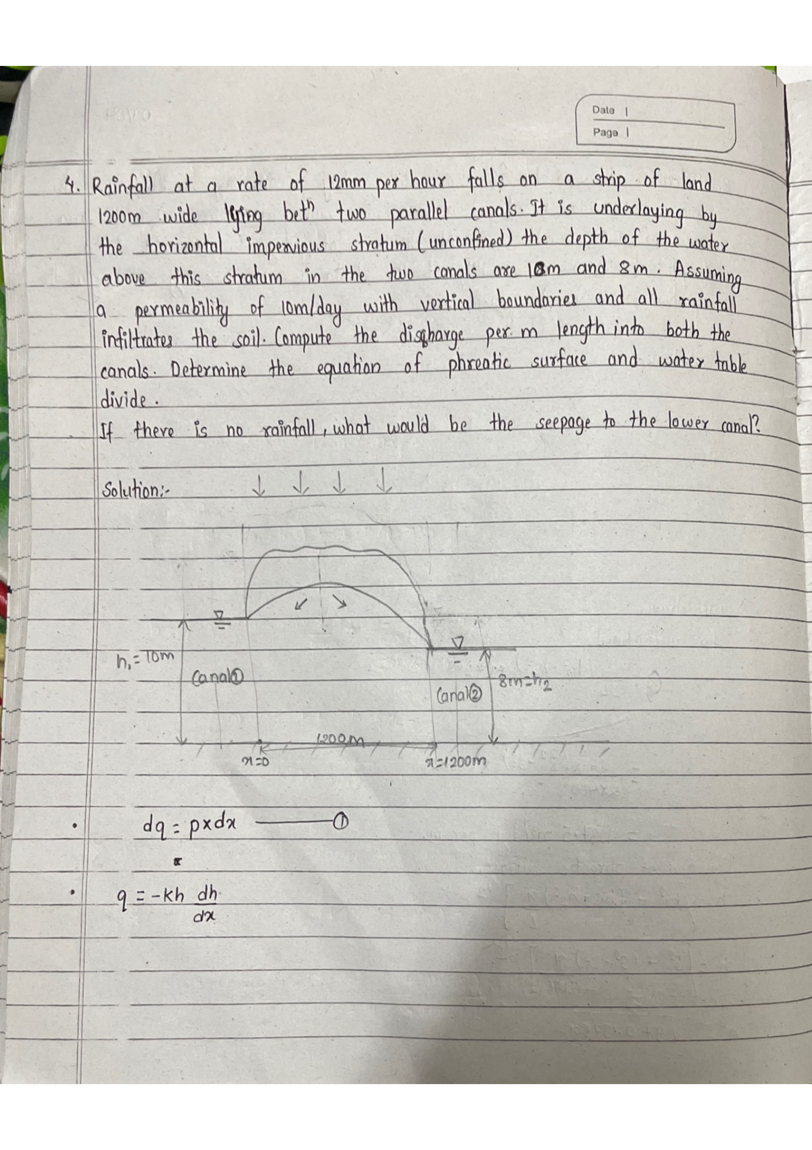
Numerical – Rainfall Between Parallel Canals

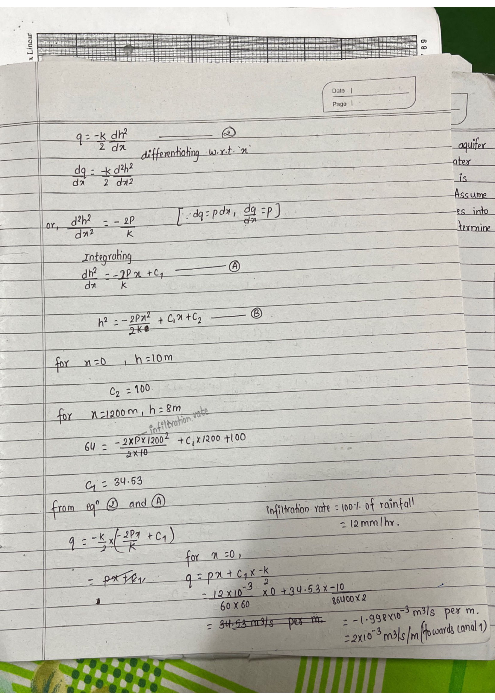
Q. Strip 1200 m wide, P = 12 mm/hr (100% infiltration), h₁ = 10 m, h₂ = 8 m, K = 10 m/day. Find discharge, phreatic surface, water divide, seepage without rainfall.

Fig: Rainfall recharging unconfined aquifer between two canals — mounded water table with divide

Solution:

Derivation: \( q = -\frac{K}{2} \frac{dh^2}{dx} \), continuity with recharge: \( \frac{dq}{dx} = P \)

\[ \frac{d^2 h^2}{dx^2} = -\frac{2P}{K} \]

Page 27

Transcription

(Continuation – Rainfall Between Parallel Canals)

Integrating twice:

\[ h^2 = -\frac{P}{K}\,x^2 + C_1 x + C_2 \]

Boundary Conditions:

x = 0, h = 10: C₂ = 100

x = 1200, h = 8:

P/K = (12 × 24)/(10 × 1000) = 0.0288

64 = −0.0288 × 1,440,000 + 1200 C₁ + 100

C₁ = 41,436/1200 = 34.53

At x = 0 (canal 1):

\[ q_1 = -\frac{K}{2} \times C_1 = -\frac{10}{172{,}800} \times 34.53 = \boxed{-1.998 \times 10^{-3} \text{ m}^3\text{/s/m}} \]

Page 28

Transcription

At x = 1200 (canal 2):

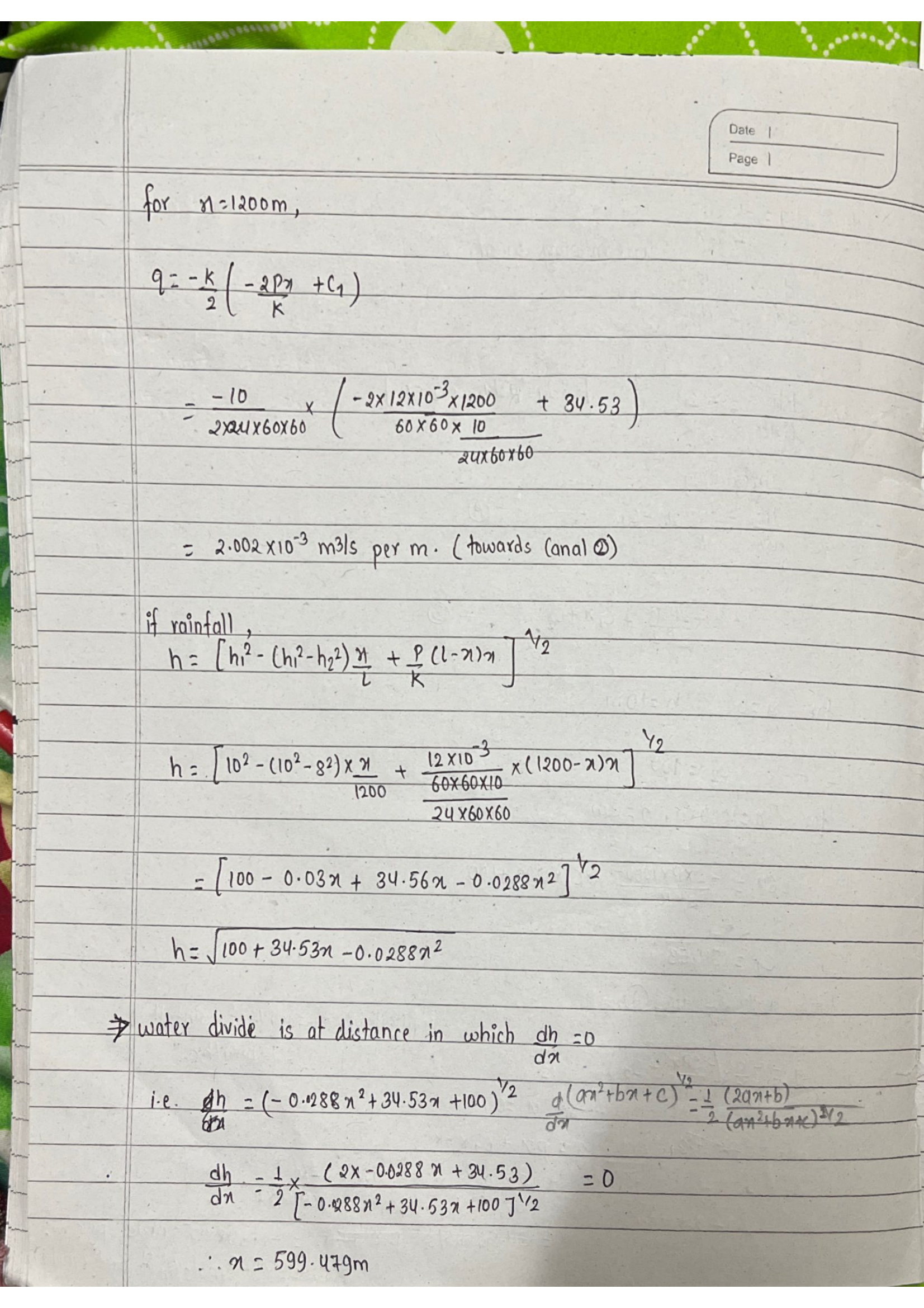
\[ q_2 = -\frac{K}{2}(-\frac{2P}{K} \times 1200 + C_1) = -\frac{10}{172{,}800}(-69.12 + 34.53) = \boxed{2.002 \times 10^{-3} \text{ m}^3\text{/s/m}} \]

Phreatic surface:

\[ h = \sqrt{100 + 34.53x - 0.0288x^2} \]

Water table divide (dh²/dx = 0):

\[ x = \frac{34.53}{0.0576} = \boxed{599.48 \text{ m from canal 1}} \]

Page 29

Transcription

Without Rainfall (P = 0):

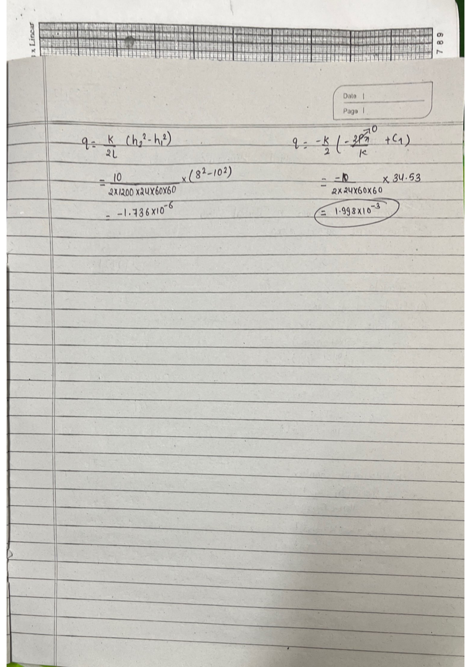
\[ q_0 = \frac{K(h_1^2 - h_2^2)}{2L} = \frac{10 \times 36}{86{,}400 \times 2400} = \boxed{1.736 \times 10^{-6} \text{ m}^3\text{/s/m}} \]

Note: Discharge without rainfall is about 1000× smaller, showing the dominant effect of recharge.

Page 30

Transcription

Date: 09/14

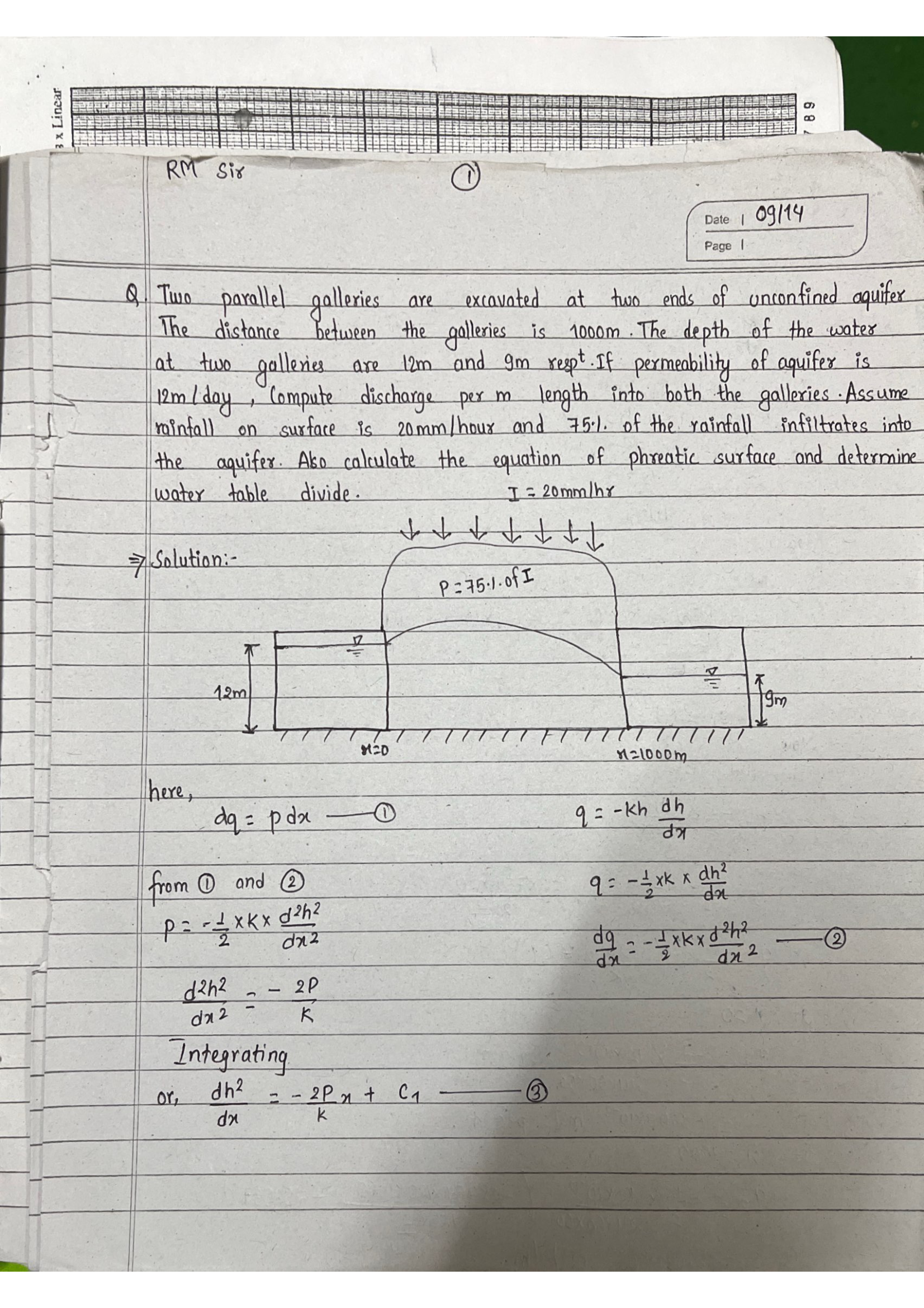
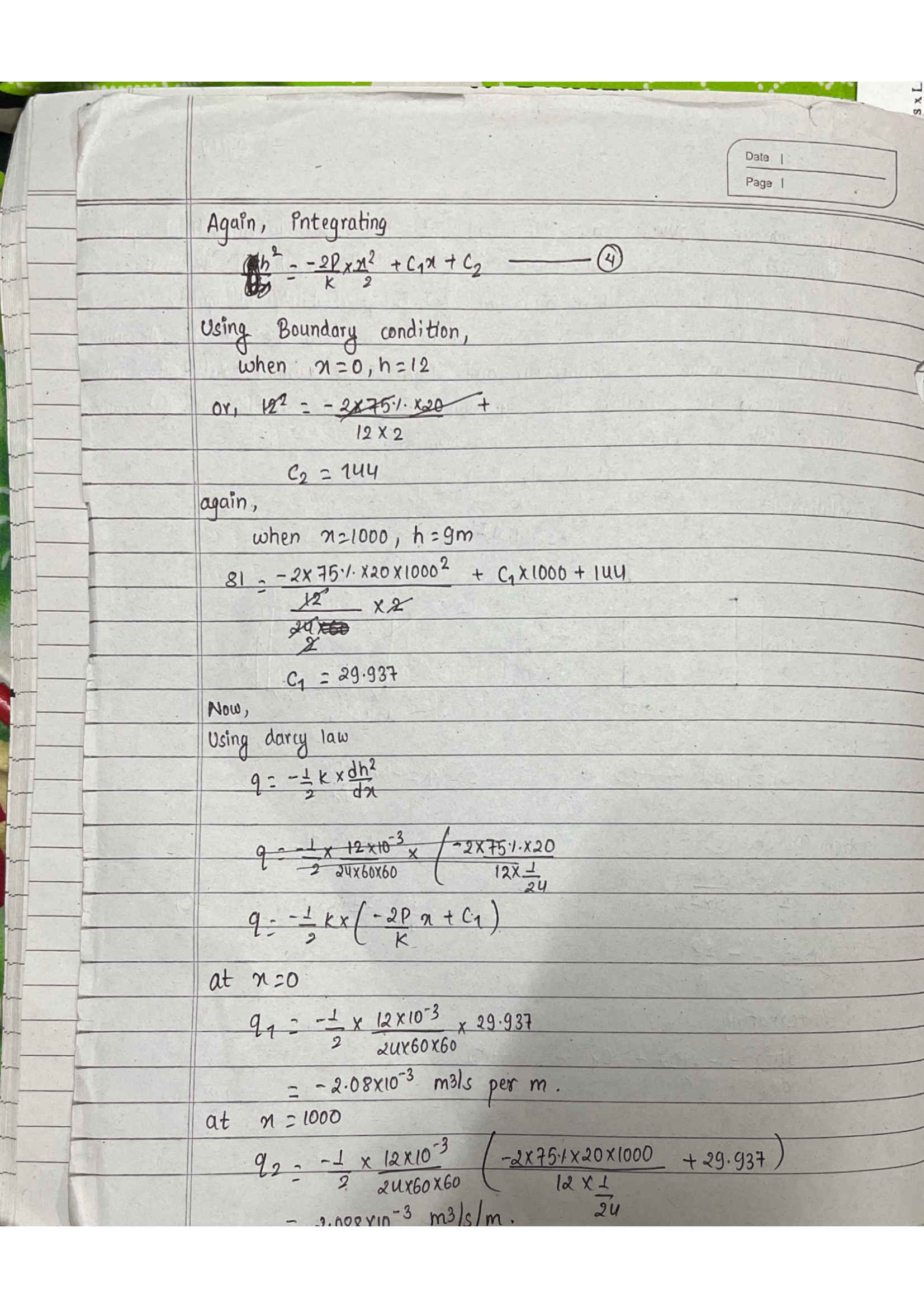
Numerical – Two Parallel Galleries (Unconfined with Rainfall)

Q. Galleries 1000 m apart, h₁ = 12 m, h₂ = 9 m, K = 12 m/day, P = 75% of 20 mm/hr = 15 mm/hr. Find discharge, phreatic surface, water divide.

Diagram: Two galleries at x=0 (h₁=12m) and x=1000m (h₂=9m), impervious stratum below, rain from above.

Solution:

\[ \frac{d^2(h^2)}{dx^2} = -\frac{2P}{K} \]

Integrating: \( h^2 = -\frac{P}{K}x^2 + C_1 x + C_2 \)

Page 31

Transcription

Boundary Conditions:

x = 0, h = 12: C₂ = 144

x = 1000, h = 9:

P/K = (15 × 24)/(12 × 1000) = 0.03

81 = −0.03 × 10⁶ + 1000 C₁ + 144

C₁ = 29,937/1000 = 29.937

Page 32

Transcription

Discharge:

At x = 0:

\[ q_1 = -\frac{12}{172{,}800} \times 29.937 = \boxed{-2.079 \times 10^{-3} \text{ m}^3\text{/s/m}} \]

At x = 1000:

\[ q_2 = -\frac{12}{172{,}800}(-60 + 29.937) = \boxed{2.088 \times 10^{-3} \text{ m}^3\text{/s/m}} \]

Check: |q₁| + |q₂| = P × L ✓

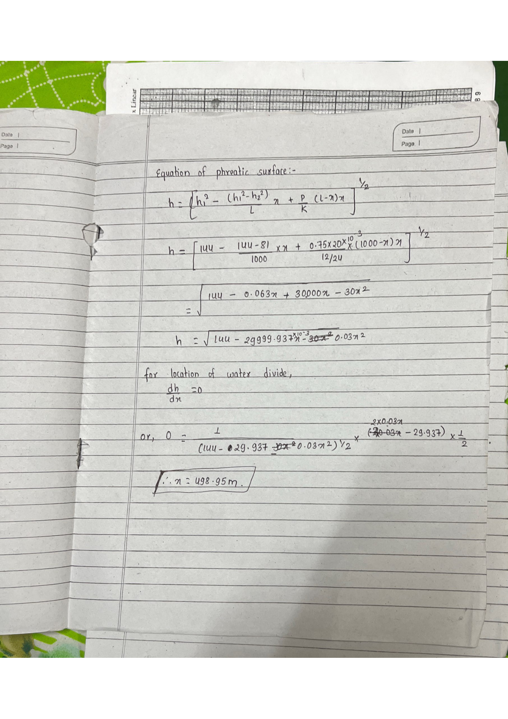
Phreatic surface:

\[ h = \sqrt{144 + 29.937x - 0.03x^2} \]

Water table divide:

\[ x = \frac{29.937}{0.06} = \boxed{498.95 \text{ m from gallery 1}} \]