← All Chapters
Summary Note 2 / 7

Chapter 1 & 2 – Numericals (Properties, Darcy's Law)

GWE Handwritten Notes

Page 10

Page 10
Transcription

Date: 2081/08/10
Page |

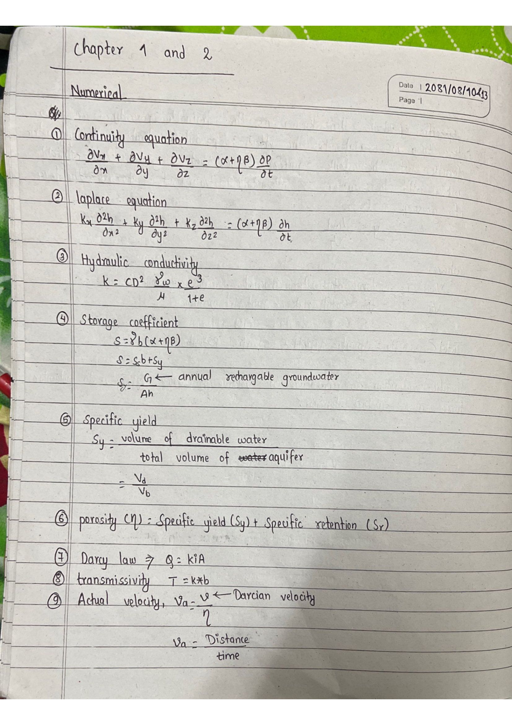
Chapter 1 and 2 – Numericals

Key Formulae

  1. Continuity equation:
    \[ \frac{\partial V_x}{\partial x} + \frac{\partial V_y}{\partial y} + \frac{\partial V_z}{\partial z} = (\alpha + \eta\beta)\frac{\partial P}{\partial t} \]

    where α = compressibility of aquifer skeleton, β = compressibility of water, η = porosity, P = pressure

  2. Laplace / Diffusion equation:
    \[ K_x \frac{\partial^2 h}{\partial x^2} + K_y \frac{\partial^2 h}{\partial y^2} + K_z \frac{\partial^2 h}{\partial z^2} = (\alpha + \eta\beta)\frac{\partial h}{\partial t} \]

    For homogeneous, isotropic, steady state: \( \nabla^2 h = 0 \) (Laplace equation)

  3. Hydraulic conductivity:
    \[ K = C D^2 \frac{\gamma_w}{\mu} \times \frac{e^3}{1+e} \]

    C = shape factor, D = effective grain diameter, γw = unit wt. of water, μ = dynamic viscosity, e = void ratio

  4. Storage coefficient:
    \[ S = \gamma_w b(\alpha + \eta\beta) \quad ; \quad S = S_s \cdot b \quad ; \quad S = \frac{G}{A \cdot \Delta h} \]

    where G = vol. of GW released/stored, A = area, Δh = change in head, b = thickness

  5. Specific yield:
    \[ S_y = \frac{V_d}{V_b} \]

    Vd = volume of water drained by gravity, Vb = bulk volume of soil

  6. Porosity:
    \[ \eta = S_y + S_r \]

    Sy = specific yield, Sr = specific retention

  7. Darcy’s law:
    \[ Q = K i A \quad ; \quad V = K i \quad ; \quad q = -K\frac{dh}{dx} \]
    Porous Medium (K = hydraulic conductivity) Q → h₁ h₂ Datum Δh L i = Δh / L (hydraulic gradient) A = cross-section area
    Fig: Darcy's Law — flow through porous medium
  8. Transmissivity:
    \[ T = K \times b \]

    K = hydraulic conductivity, b = aquifer thickness

  9. Actual velocity (Seepage velocity):
    \[ V_a = \frac{V}{\eta} = \frac{Ki}{\eta} \]
Page 11

Page 11
Transcription

Date |
Page |

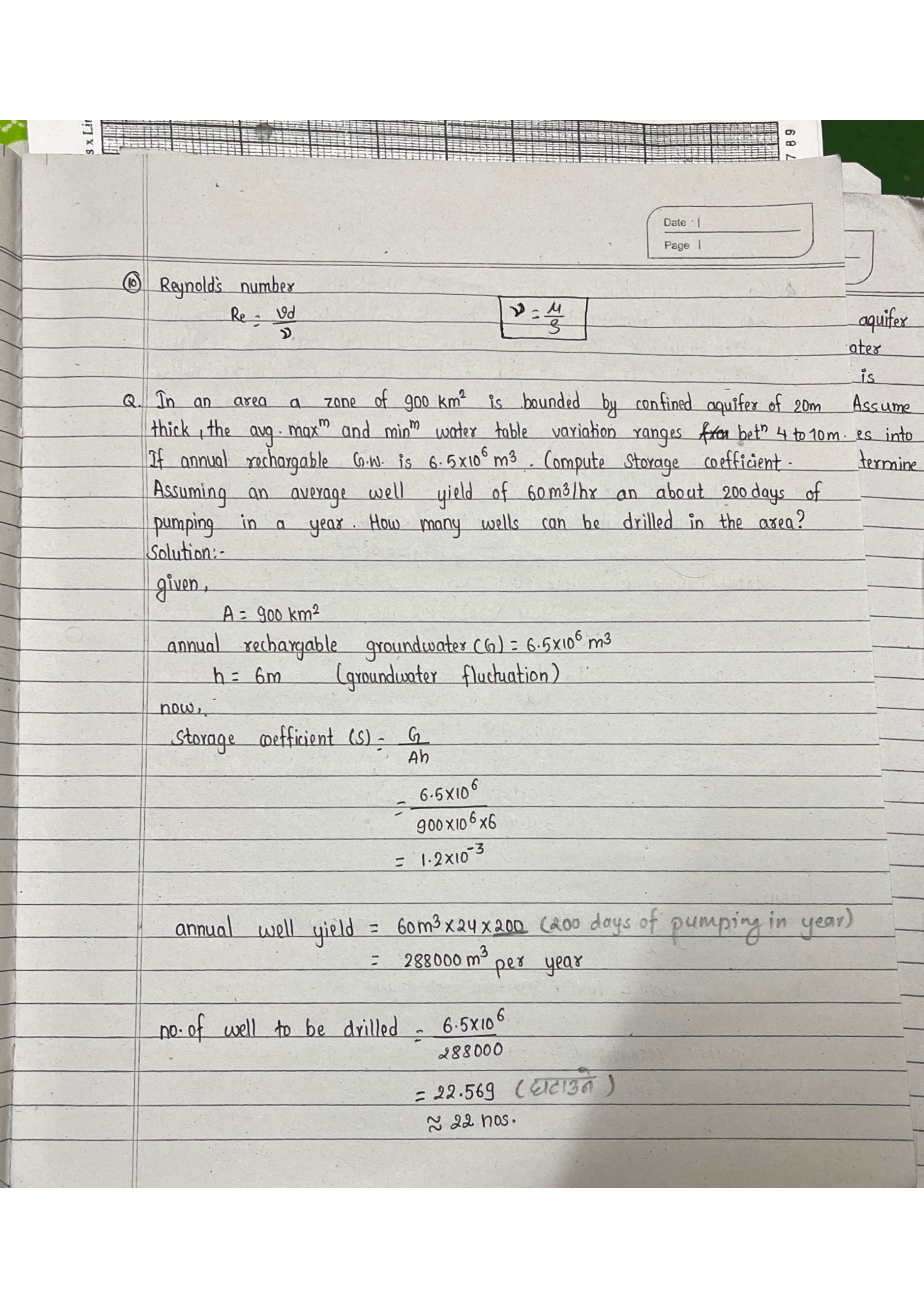
Reynolds Number

\[ Re = \frac{V \cdot d}{\nu} \qquad \text{where } \nu = \frac{\mu}{\rho} \]

V = Darcy velocity, d = grain diameter, ν = kinematic viscosity, μ = dynamic viscosity, ρ = density of water

  • If Re < 1 → Laminar flow → Darcy’s law is valid
  • If Re > 10 → Turbulent flow → Darcy’s law is not valid

Numerical 1

Q. An area of 900 km² is underlain by a confined aquifer of 20 m thickness. The groundwater table fluctuates between 4 m and 10 m. The annual rechargeable groundwater volume is 6.5 × 10⁶ m³. Compute the storage coefficient (S). If the well yield is 60 m³/hr and pumping is for 200 days per year, how many wells can be supported?

Ground Surface Confining Layer (Aquitard) Confined Aquifer (b = 20 m) Bedrock Piezo. h b A = 900 km², Δh = 6 m
Fig: Confined aquifer — storage coefficient concept

Given:

  • A = 900 km² = 900 × 106 m²
  • b = 20 m
  • Δh = 10 − 4 = 6 m
  • G = 6.5 × 10⁶ m³ (annual rechargeable GW volume)
  • Well yield = 60 m³/hr
  • Pumping period = 200 days/year

Solution:

(i) Storage coefficient:

Concept: S = volume of water released per unit surface area per unit decline in head.

\[ S = \frac{G}{A \times \Delta h} \]

Substituting values:

\[ S = \frac{6.5 \times 10^6}{900 \times 10^6 \times 6} = \frac{6.5}{5400} = \mathbf{1.2 \times 10^{-3}} \]

Check: S is in the range 10−5 to 10−3 for confined aquifers. ✓

(ii) Number of wells:

Step 1 — Compute annual yield per well:

\[ Q_{\text{well}} = 60 \;\text{m}^3/\text{hr} \times 24\;\text{hr/day} \times 200\;\text{days/yr} = 288{,}000\;\text{m}^3/\text{yr} \]

Step 2 — Divide available recharge by per-well yield:

\[ \text{No. of wells} = \frac{G}{Q_{\text{well}}} = \frac{6.5 \times 10^6}{288{,}000} = 22.57 \approx \mathbf{22 \text{ nos.}} \]

(Take floor value to ensure sustainable pumping ≤ recharge.)

Page 12

Page 12
Transcription

Date |
Page |

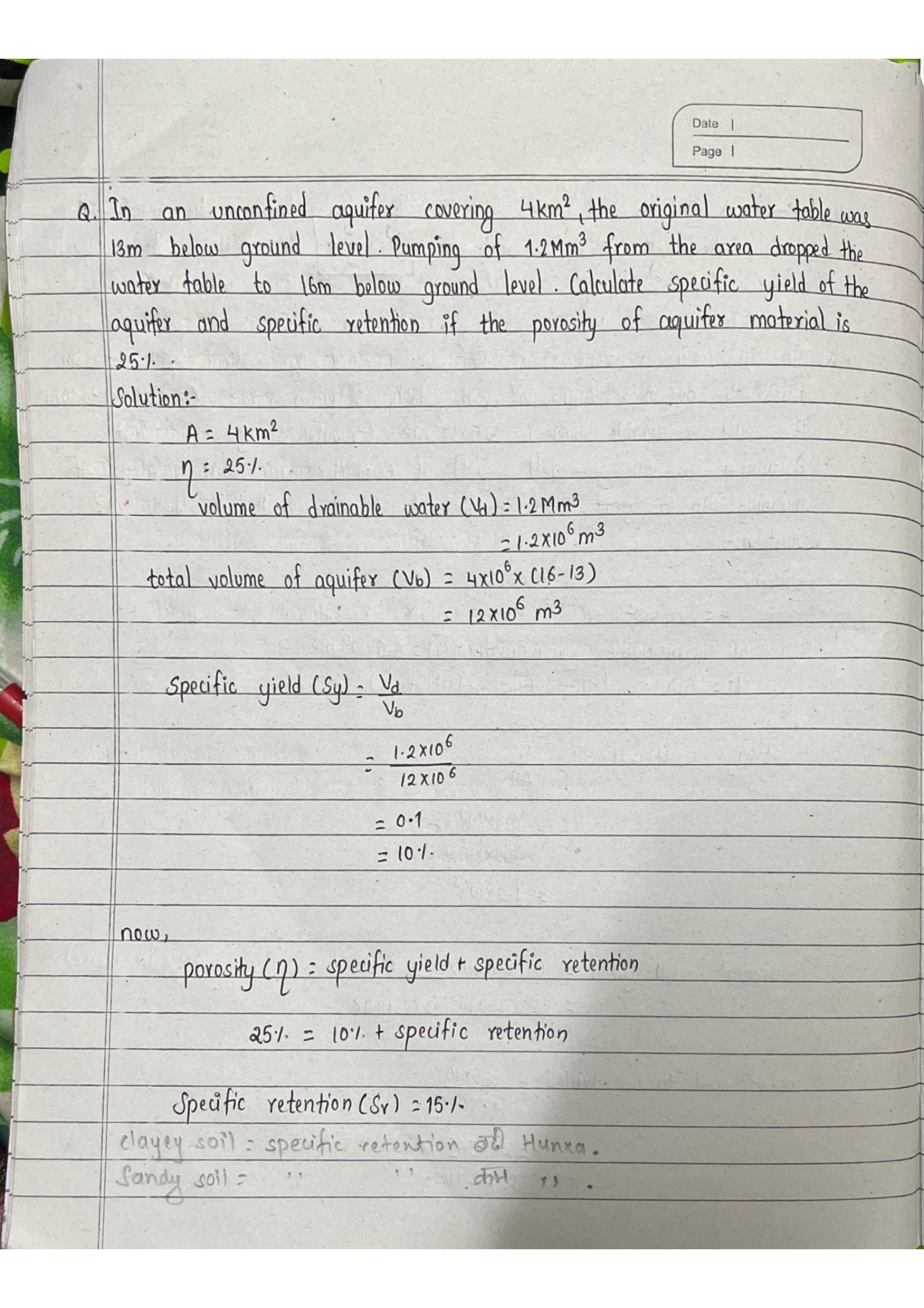
Numerical 2

Q. An unconfined aquifer of area 4 km² has its water level dropped from 13 m to 16 m below ground level (BGL) after pumping 1.2 Mm³ (million m³) of water. Find the specific yield Sy and specific retention Sr if porosity η = 25%.

Ground Level WT (before) WT (after) Dewatered zone (Δh = 3 m) Saturated Zone 13 m 16 m A = 4 km²
Fig: Water table drop in unconfined aquifer

Given:

  • A = 4 km² = 4 × 10⁶ m²
  • Drop in WL = 16 − 13 = 3 m (Δh = 3 m)
  • Volume pumped Vd = 1.2 × 10⁶ m³ = 1.2 Mm³
  • η = 25%

Solution:

Step 1 — Bulk volume of aquifer dewatered:

\[ V_b = A \times \Delta h = 4 \times 10^{6} \times 3 = 12 \times 10^{6}\;\text{m}^3 \]

Step 2 — Specific yield (ratio of drainable water to bulk volume):

\[ S_y = \frac{V_d}{V_b} = \frac{1.2 \times 10^6}{12 \times 10^6} = 0.10 = \mathbf{10\%} \]

Step 3 — Specific retention (water retained against gravity):

\[ \eta = S_y + S_r \implies S_r = 25\% - 10\% = \mathbf{15\%} \]

Note: Clayey soil → high Sr ; Sandy soil → low Sr. Here Sr > Sy, suggesting a finer-grained material.

Page 13

Page 13
Transcription

Date |
Page |

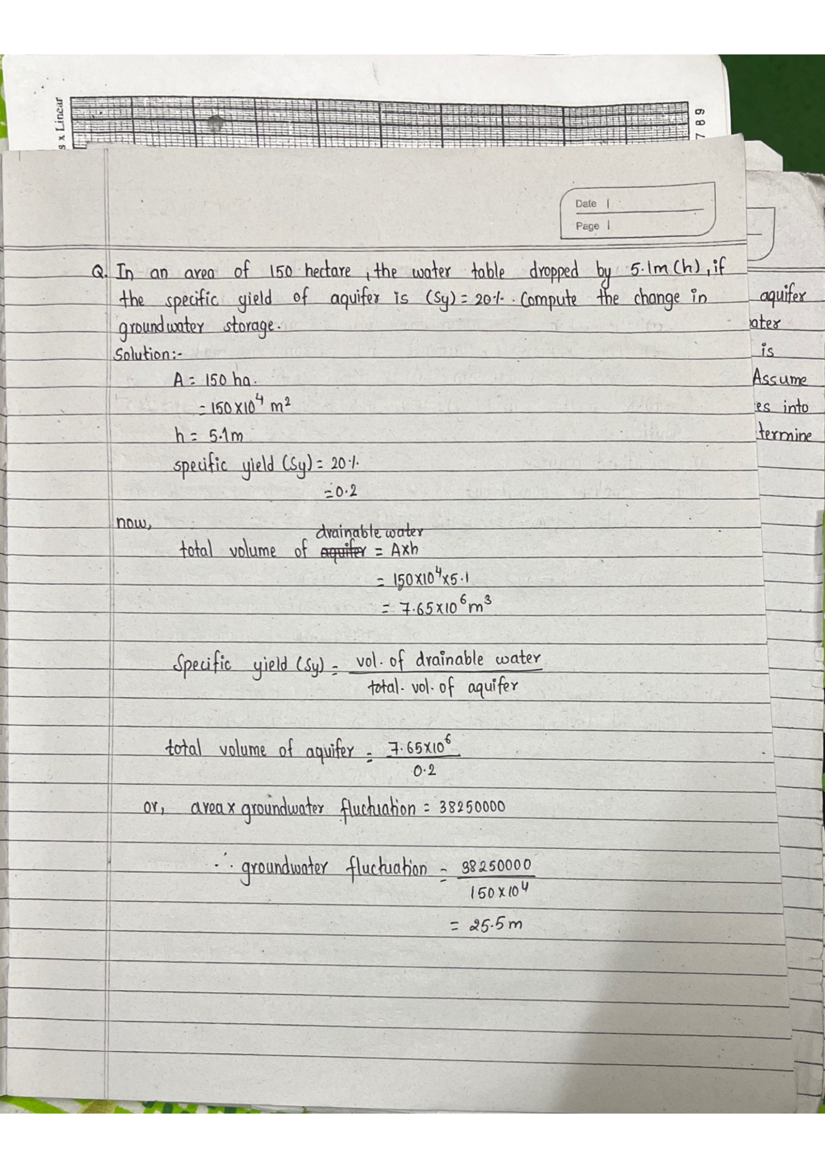
Numerical 3

Q. A volume of 7.65 × 10⁶ m³ of water was pumped from an unconfined aquifer of area 150 ha. If Sy = 20%, compute the change in groundwater level (GW fluctuation).

Given:

  • A = 150 ha = 150 × 104 m² = 1.5 × 10⁶ m²
  • Vd = 7.65 × 10⁶ m³
  • Sy = 20% = 0.20

Solution:

Volume of drainable water per unit area:

Vd / A = 7.65 × 10⁶ / (150 × 104) = 5.1 m

Check: 150 × 104 × 5.1 = 7.65 × 10⁶ m³ ✓

Total volume of aquifer dewatered:

\[ V_b = \frac{V_d}{S_y} = \frac{7.65 \times 10^6}{0.2} = 38{,}250{,}000 \text{ m}^3 \]

GW fluctuation (drop in water table):

\[ \Delta h = \frac{V_b}{A} = \frac{38{,}250{,}000}{150 \times 10^4} = \mathbf{25.5 \text{ m}} \]

Or equivalently: Δh = 5.1 / Sy = 5.1 / 0.2 = 25.5 m

Page 14

Page 14
Transcription

Date |
Page |

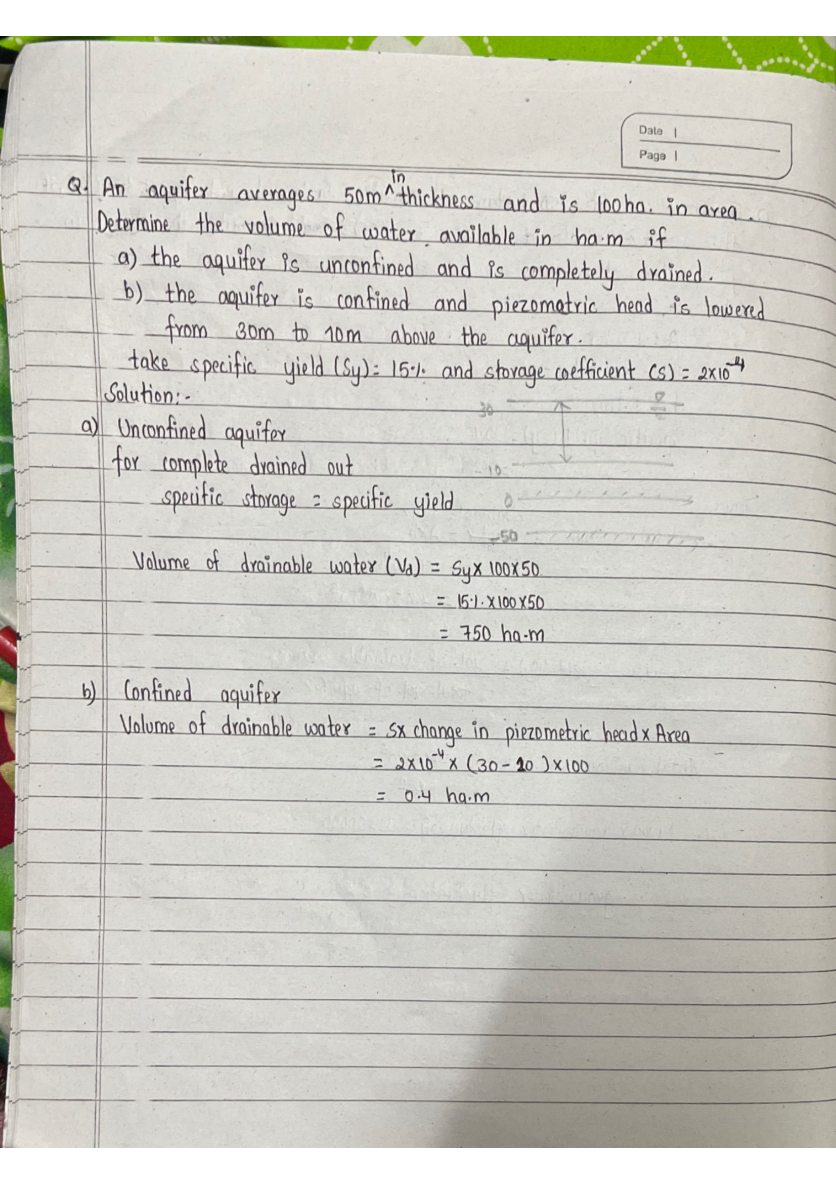
Numerical 4

Q. An aquifer 50 m thick covers an area of 100 ha. Find the volume of water available if:

  1. It is an unconfined aquifer and is completely drained.
  2. It is a confined aquifer and the piezometric head is lowered from 30 m to 10 m.

Given: Sy = 15%, S = 2 × 10⁻⁴

(a) Unconfined GL b = 50 m Completely drained V = Sᵧ × A × b = 750,000 m³ (b) Confined b = 50 m Δh=20m Aquifer stays saturated V = S × A × Δh = 4,000 m³
Fig: Comparison — unconfined yields 187× more water than confined for same aquifer

Given:

  • b = 50 m (aquifer thickness)
  • A = 100 ha = 100 × 104 m² = 106 m²
  • Sy = 15% = 0.15 (for unconfined)
  • S = 2 × 10⁻⁴ (for confined)
  • Δh = 30 − 10 = 20 m (for confined)

Solution:

a) Unconfined aquifer (completely drained):

For unconfined, drainable volume = Sy × A × (saturated thickness drained):

\[ V_d = S_y \times A \times b = 0.15 \times 10^6 \times 50 = 7{,}500{,}000\;\text{m}^3 \]

Converting: 7,500,000 / 104 = 750 ha·m

b) Confined aquifer (head lowered 30 → 10 m):

For confined, water released = S × A × Δh (storage coefficient governs):

\[ V_d = S \times A \times \Delta h = 2 \times 10^{-4} \times 10^6 \times 20 = 4{,}000\;\text{m}^3 \]

Converting: 4,000 / 104 = 0.4 ha·m

Key insight: Confined aquifer yields much less water per unit head change compared to unconfined aquifer because S ≪ Sy (factor of ~750). In confined aquifers, water is released by compression of the aquifer skeleton and expansion of water, not by actual drainage of pores.

Page 15

Page 15
Transcription

Date |
Page |

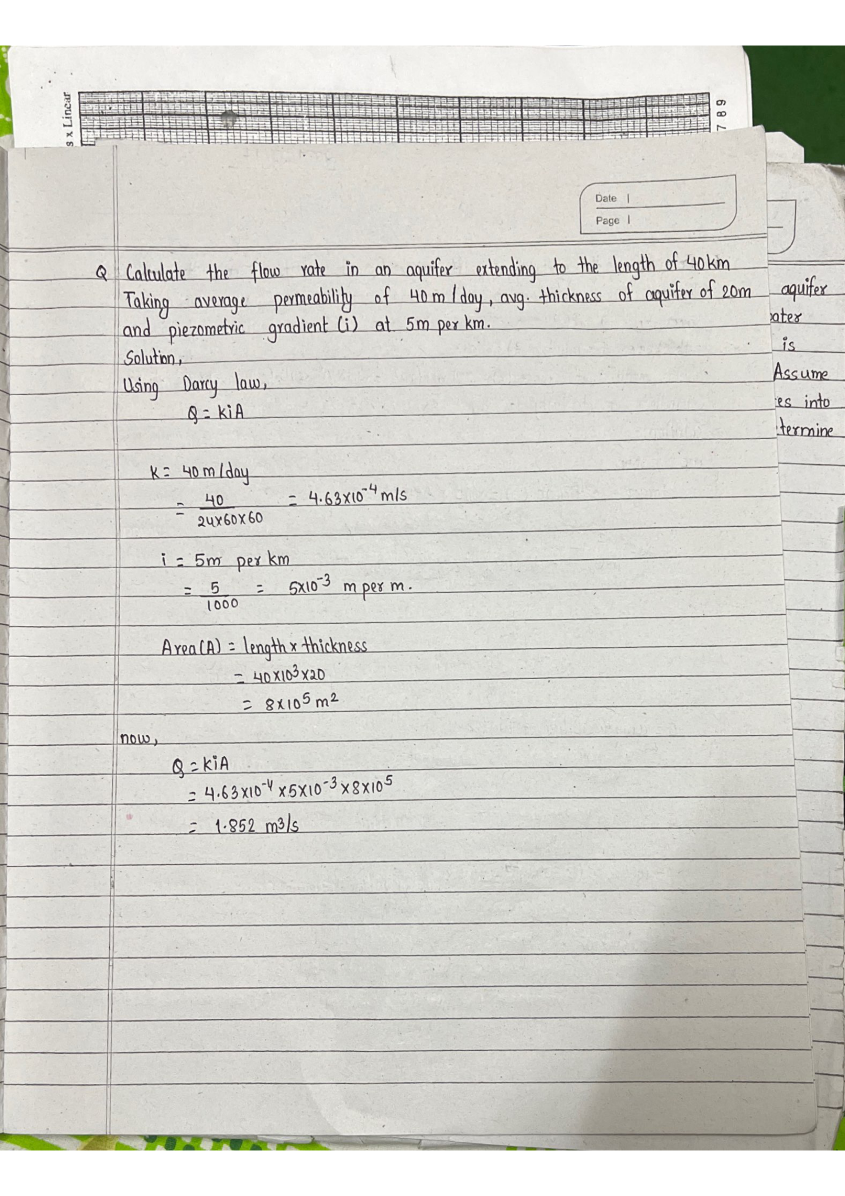
Numerical 5

Q. An aquifer has a length of 40 km, hydraulic conductivity K = 40 m/day, thickness b = 20 m, and hydraulic gradient i = 5 m/km. Find the flow rate Q.

Given:

  • Length (width of cross-section) = 40 km = 40,000 m
  • K = 40 m/day
  • b = 20 m
  • i = 5 m/km = 5/1000 = 5 × 10⁻³

Solution:

Convert K to m/s:

K = 40 / (24 × 3600) = 40 / 86400 = 4.63 × 10⁻⁴ m/s

Cross-sectional area perpendicular to flow:

A = length × thickness = 40,000 × 20 = 800,000 m² = 8 × 10⁵ m²

Applying Darcy’s law:

\[ Q = K \cdot i \cdot A = 4.63 \times 10^{-4} \times 5 \times 10^{-3} \times 8 \times 10^{5} \]

= 4.63 × 5 × 8 × 10(−4−3+5)

= 185.2 × 10⁻²

\[ Q = \mathbf{1.852 \text{ m}^3/\text{s}} \]

Page 16

Page 16
Transcription

2081/08/17   Page

Numerical 6

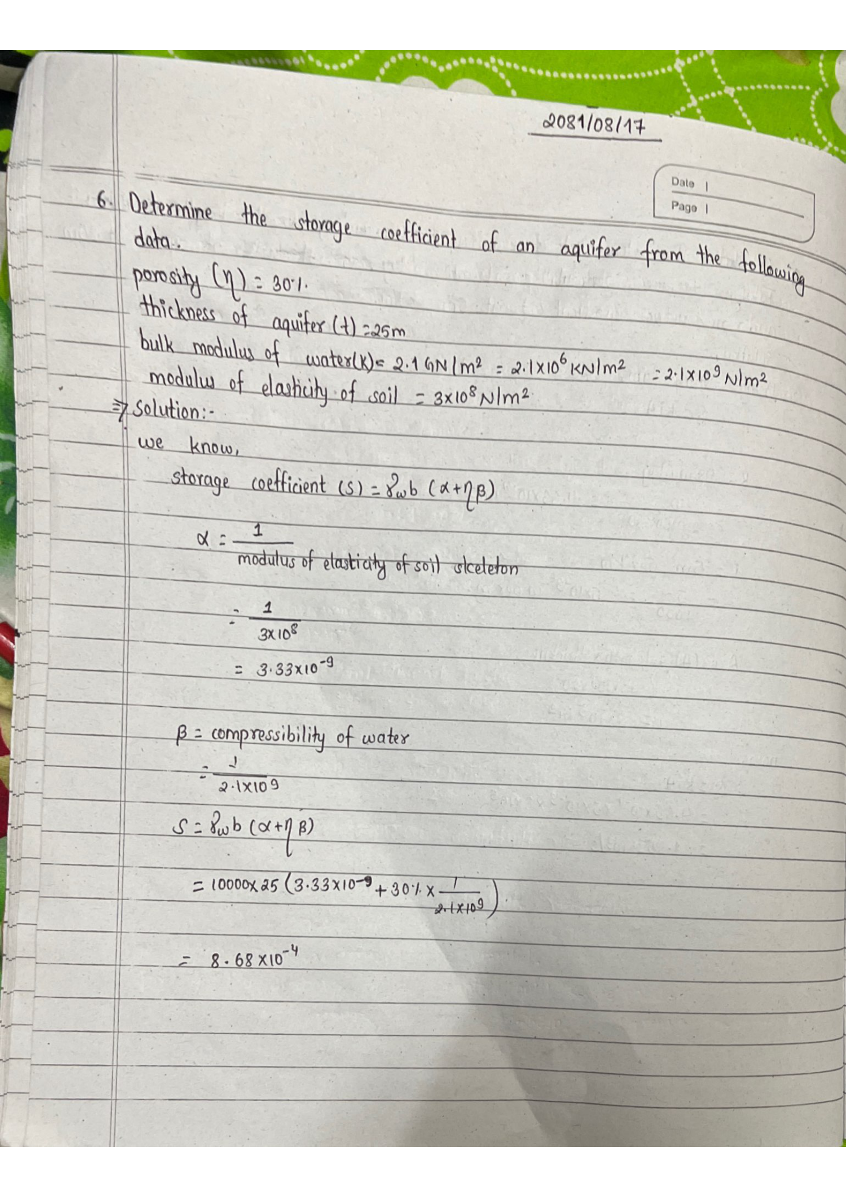
Q. Determine the storage coefficient of an aquifer from the following data:

  • porosity (\(\eta\)) = 30%
  • thickness of aquifer (\(b\)) = 25 m
  • bulk modulus of water (\(K_w\)) = 2.1 GN/m² = 2.1 × 10⁹ N/m²
  • modulus of elasticity of soil = 3 × 10⁸ N/m²

Solution:

Step 1 — Identify the formula. For a confined aquifer:

\[ S = \gamma_w \cdot b \left( \alpha + \eta \beta \right) \]

where γw = 9810 N/m³ ≈ 104 N/m³

Step 2 — Compute compressibility of aquifer skeleton (α):

\[ \alpha = \frac{1}{E_{\text{soil}}} = \frac{1}{3 \times 10^{8}} = 3.33 \times 10^{-9} \;\text{m}^{2}\text{/N} \]

Step 3 — Compute compressibility of water (β):

\[ \beta = \frac{1}{K_w} = \frac{1}{2.1 \times 10^{9}} = 4.76 \times 10^{-10} \;\text{m}^{2}\text{/N} \]

Step 4 — Compute (α + ηβ):

\[ \alpha + \eta\beta = 3.33 \times 10^{-9} + 0.30 \times 4.76 \times 10^{-10} = 3.33 \times 10^{-9} + 1.43 \times 10^{-10} \] \[ = 3.473 \times 10^{-9} \;\text{m}^2/\text{N} \]

Step 5 — Compute S:

\[ S = 10{,}000 \times 25 \times 3.473 \times 10^{-9} = \mathbf{8.68 \times 10^{-4}} \]

Check: S is in the range 10−5 to 10−3 for confined aquifers. ✓

Note: α ≫ ηβ here, meaning aquifer skeleton compressibility dominates over water compressibility.

Page 17

Page 17
Transcription

Numerical 7

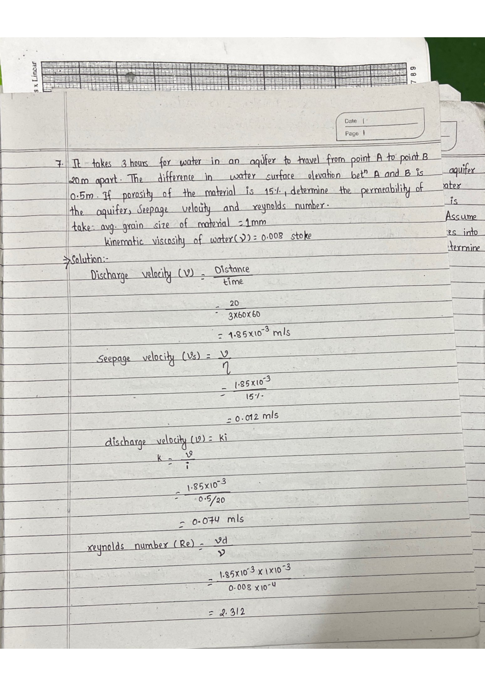
Q. It takes 3 hours for water in an aquifer to travel from point A to point B, 20 m apart. The difference in water surface elevation between A and B is 0.5 m. If porosity of the material is 15%, determine the permeability of the aquifer, seepage velocity and reynolds number.

Take: avg. grain size of material = 1 mm, kinematic viscosity of water (\(\nu\)) = 0.008 stoke

Solution:

Discharge velocity:

\[ V = \frac{20}{3 \times 60 \times 60} = 1.85 \times 10^{-3} \text{ m/s} \]

Seepage velocity:

\[ V_s = \frac{V}{\eta} = \frac{1.85 \times 10^{-3}}{0.15} = \mathbf{0.012 \text{ m/s}} \]

Permeability:

\[ k = \frac{V}{i} = \frac{1.85 \times 10^{-3}}{0.5 / 20} = \frac{1.85 \times 10^{-3}}{0.025} = \mathbf{0.074 \text{ m/s}} \]

Reynolds number:

\[ Re = \frac{V \cdot d}{\nu} = \frac{1.85 \times 10^{-3} \times 1 \times 10^{-3}}{0.008 \times 10^{-4}} = \mathbf{2.312} \]

Page 18

Page 18
Transcription

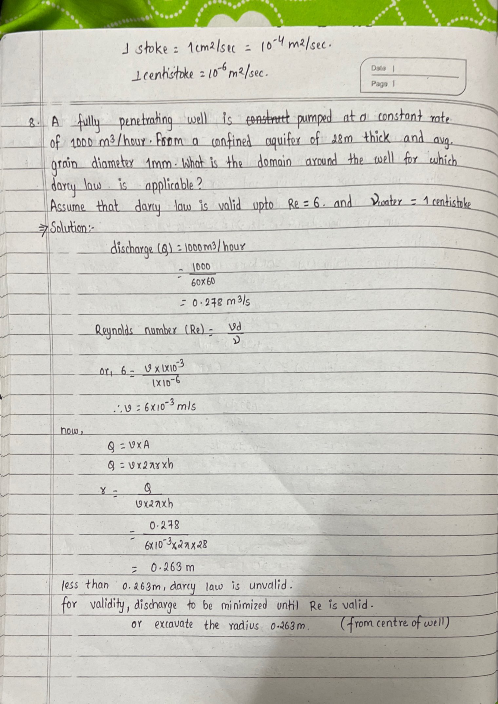
1 stoke = 1 cm²/sec = 10−4 m²/sec

1 centistoke = 10−6 m²/sec

Numerical 8

Q. A fully penetrating well is constructed & pumped at a constant rate of 1000 m³/hour from a confined aquifer of 28 m thick and avg. grain diameter 1 mm. What is the domain around the well for which Darcy law is applicable?

Assume that Darcy law is valid upto Re = 6 and \(\nu_{\text{water}}\) = 1 centistoke

Plan View Darcy's law VALID (Re < 6) INVALID Re > 6 Well r = 0.263 m Q (inflow)
Fig: Domain of Darcy's law validity around a pumping well

Solution:

Step 1 — Convert discharge to m³/s:

\[ Q = \frac{1000}{3600} = 0.278 \;\text{m}^{3}\text{/s} \]

Step 2 — Find limiting Darcy velocity from Re condition:

At the critical radius, Re = 6 (maximum for Darcy validity):

\[ Re = \frac{V \cdot d}{\nu} \quad\Rightarrow\quad 6 = \frac{V \times 10^{-3}}{10^{-6}} \quad\Rightarrow\quad V = 6 \times 10^{-3} \;\text{m/s} \]

Step 3 — Find critical radius using radial flow equation:

For a fully penetrating well in a confined aquifer, flow converges radially through a cylindrical surface of area \(2\pi r h\):

\[ Q = V \times 2\pi r \times h \quad\Rightarrow\quad r = \frac{Q}{V \times 2\pi \times h} \]
\[ r = \frac{0.278}{6 \times 10^{-3} \times 2\pi \times 28} = \frac{0.278}{1.0556} = \mathbf{0.263 \;\text{m}} \]

Interpretation: Within 0.263 m from the well centre, velocity is too high (Re > 6) and flow becomes turbulent — Darcy’s law is invalid in this zone.

Beyond 0.263 m, velocity decreases (spreading over larger area) and Darcy’s law applies.

Page 19

Page 19
Transcription

Numerical 9

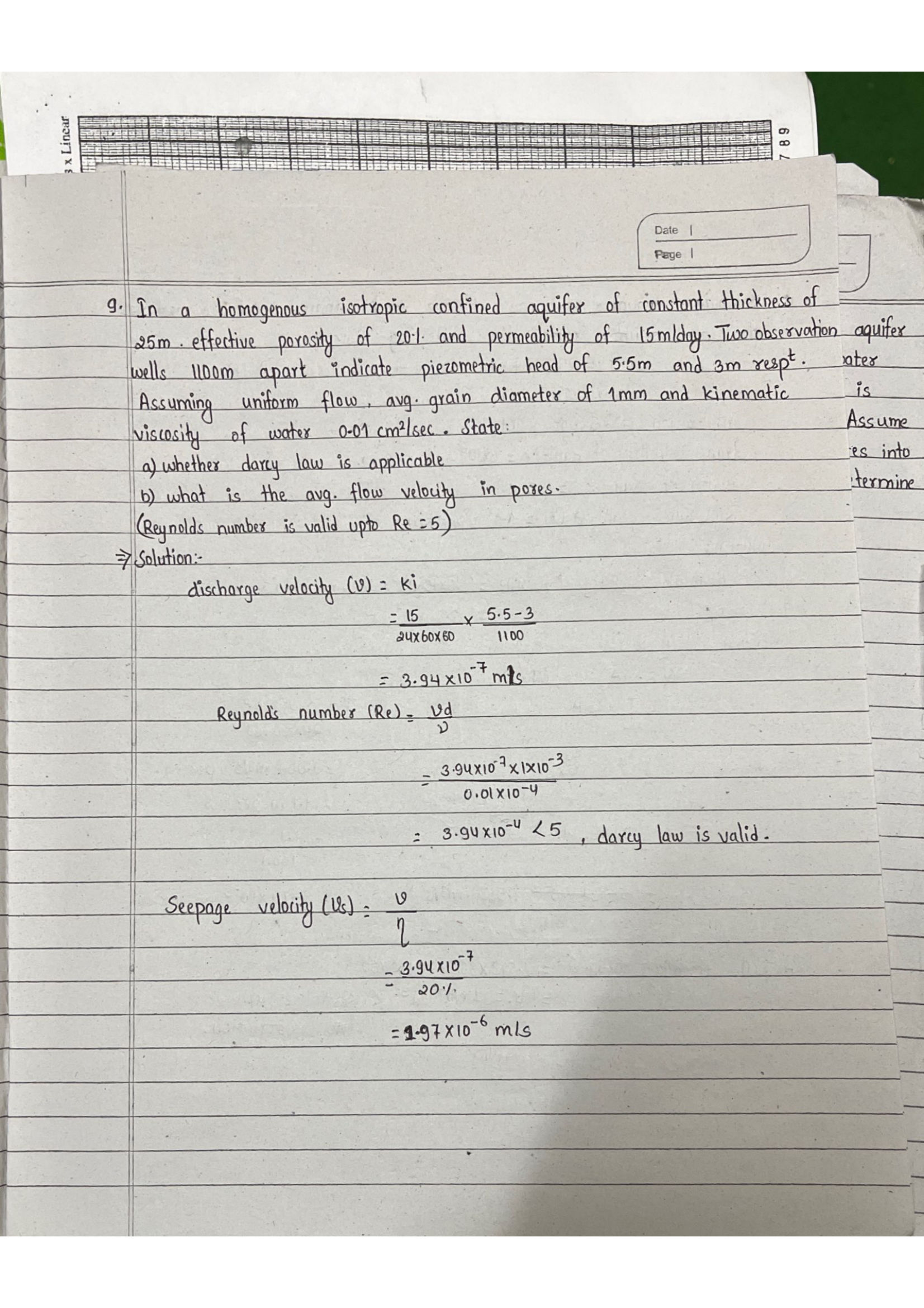
Q. In a homogeneous isotropic confined aquifer of constant thickness of 25 m, effective porosity of 20% and permeability of 15 m/day. Two observation wells 1100 m apart indicate piezometric head of 5.5 m and 3 m respectively. Assuming uniform flow, avg. grain diameter of 1 mm and kinematic viscosity of water 0.01 cm²/sec. State:

  1. whether Darcy law is applicable
  2. what is the avg. flow velocity in pores.

(Reynolds number is valid upto Re = 5)

Solution:

a) Discharge velocity:

\[ V = Ki = \frac{15}{86400} \times \frac{5.5 - 3}{1100} = 1.736 \times 10^{-4} \times 2.273 \times 10^{-3} = 3.94 \times 10^{-7} \text{ m/s} \]

Reynolds number:

\[ Re = \frac{V \cdot d}{\nu} = \frac{3.94 \times 10^{-7} \times 10^{-3}}{0.01 \times 10^{-4}} = 3.94 \times 10^{-4} \]

Since \(Re = 3.94 \times 10^{-4} < 5\), Darcy law is valid.

b) Seepage velocity:

\[ V_s = \frac{V}{\eta} = \frac{3.94 \times 10^{-7}}{0.20} = \mathbf{1.97 \times 10^{-6} \text{ m/s}} \]

Page 20

Page 20
Transcription

Numerical 10

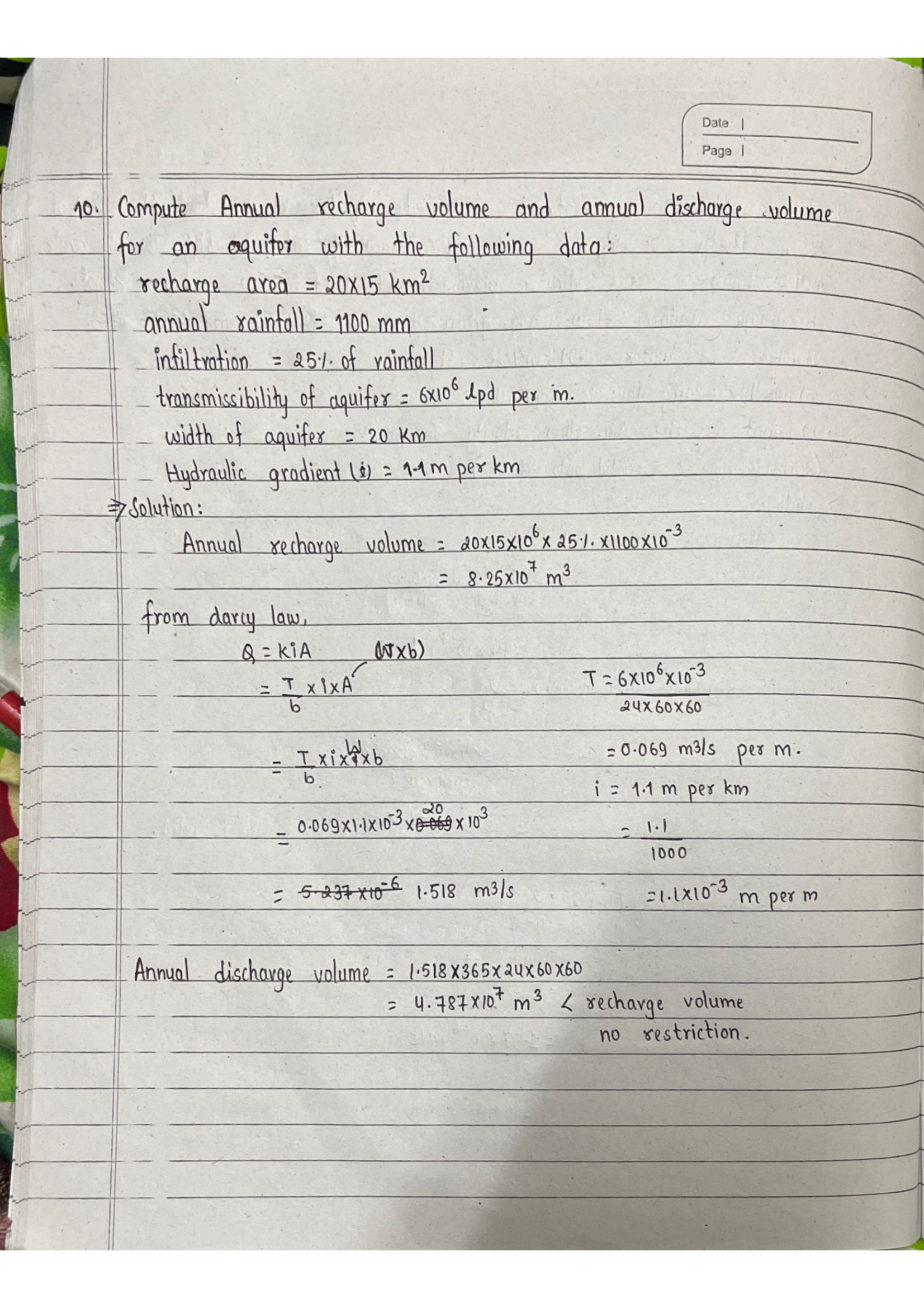
Q. Compute Annual recharge volume and annual discharge volume for an aquifer with the following data:

  • Recharge area = 20 × 15 km²
  • Annual rainfall = 1100 mm
  • Infiltration = 25% of rainfall
  • Transmissibility of aquifer = 6 × 10⁶ lpd per m
  • Width of aquifer = 20 km
  • Hydraulic gradient (\(i\)) = 1.1 m per km

Solution:

Part 1: Annual recharge volume

Step 1 — Recharge area = 20 × 15 = 300 km² = 300 × 106 m²

Step 2 — Rainfall volume = Area × annual rainfall = 300 × 106 × 1.1 = 3.3 × 10⁸ m³

Step 3 — Infiltration = 25% of rainfall:

\[ V_{\text{recharge}} = 0.25 \times 3.3 \times 10^{8} = \mathbf{8.25 \times 10^{7}\;\text{m}^{3}} \]

Part 2: Annual discharge volume

Step 1 — Convert transmissivity T from lpd/m to m²/s:

\[ T = \frac{6 \times 10^{6} \;\text{l/day/m} \times 10^{-3}\;\text{m}^3\text{/l}}{86{,}400\;\text{s/day}} = 0.0694\;\text{m}^{2}\text{/s} \]

Step 2 — Convert hydraulic gradient:

\( i = 1.1\;\text{m/km} = 1.1 / 1000 = 1.1 \times 10^{-3} \)

Step 3 — Apply Darcy’s law (Q = T × i × W):

\[ Q = 0.0694 \times 1.1 \times 10^{-3} \times 20{,}000 = 1.527\;\text{m}^{3}\text{/s} \]

Step 4 — Annual discharge = Q × seconds in a year:

\[ = 1.527 \times 365 \times 86{,}400 = \mathbf{4.816 \times 10^{7}\;\text{m}^{3}} \]

\( 4.816 \times 10^{7} < 8.25 \times 10^{7} \) (recharge volume)

∴ Annual discharge < Annual recharge — the aquifer is sustainably recharged with no over-exploitation.