Traffic Studies and Analysis

Introduction to Traffic Studies

Course Objectives and Syllabus

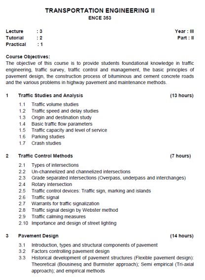
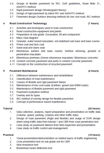
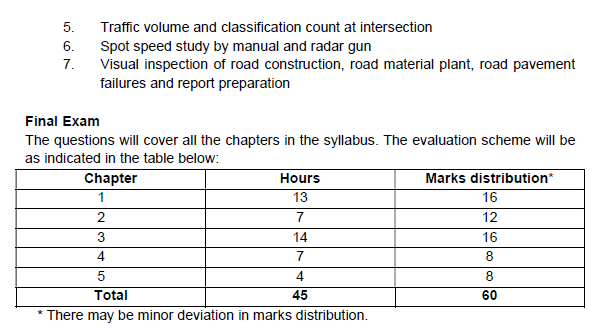
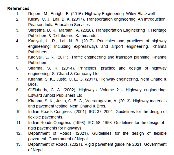
Internal evaluation: Attendance (4), Assignments and traffic data collection analysis reporting, pavement design (10) Others case study group projects for pavement failure and traffic control and management (6), Midterms (20)

Traffic Studies

• Gathering of traffic data and its inventories
• Help in planning, geometric design, traffic control and economic studies for safe and efficient movements of traffic

Need of Traffic Studies

• To investigate the current trend of traffic characteristics
• To evaluate traffic performance of the system
• To predict future traffic behavior
• To understand the needs and choices of public private sector for mobility
• To assess and prioritize potential improvements (new developments, alteration in design/traffic control and regulations etc.)

Various Traffic Studies

1. Traffic Volume Studies
2. Traffic Speed and Delay Studies
3. Origin and Destination Study
4. Basic Traffic Flow Parameters
5. Traffic Capacity and Level of Service
6. Parking Studies
7. Crash Studies

1.1 Traffic Volume Studies

Traffic Volume

• Number of vehicles that pass a point on a highway or a given lane or direction of a highway during a specified time interval.
• A quantity measure of flow
• ‘vehicles’ although often expressed as vehicles per unit time, Eg. veh/hr, veh/day

Traffic Volume Study

• Volume study is a process of counting traffic volume on a highway facility as a way of determining the traffic demand, which is an input for all traffic engineering tasks
• Complete volume study includes classified volume study recording:
  • Volume of different types/classes of traffic
  • Directional distribution
  • Turning movement
  • Distribution on different lane

Objectives or Uses of Traffic Volume Studies

To evaluate and analyze existing facilities, and plan and prioritize improvements

• Classified volume study for structural design of pavement and geometric design of road
• Volume distribution study for planning regulatory measures such as one way street
• Turning movement study for planning and design of intersections and traffic controls
• Pedestrian volume study for planning and design of pedestrian facilities

Traffic Count Periods

• Short term (one hour or more)
• Full day (24 hours)
• Full week count
• Continuous count

Methods of Traffic Count

• Manual Method
• Automatic Method
• Video Taping Method
• Photographic Method
• Moving Observer (Floating Car) Technique

Manual Method

• Simplest and basic volume count procedure
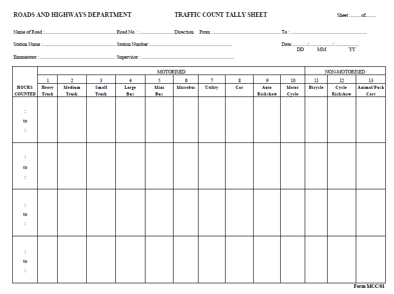
• Observer records the passage of each vehicle/pedestrian in standard sheets according to its classifications, travel direction and turning movements.

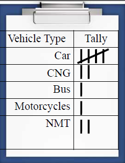
• Tallies are used.
• Typically used for periods of less than a day

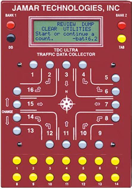
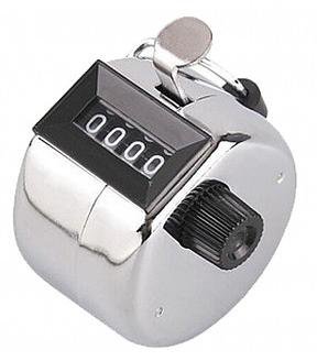
• Mechanical hand counters

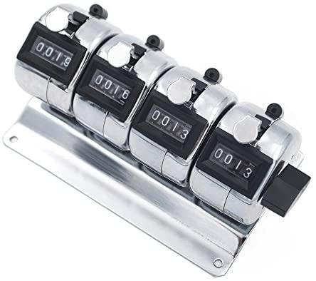
• Advantages:
  • Classification, directional and turning movement count can be obtained
  • Reliable
  • Less office work
  • Costly and sophisticated equipment are not necessary

• Disadvantages
  • Subjected to human error
  • Labor intensive
  • Not suitable for long period of count

Automatic Method

• Automatically record the total number of vehicles crossing a section of the road in a desired period
• Contact-based system:
  • Involves laying of detector such as pneumatic tube or piezoelectric strips or magnetic loop detector across a road which are connected to a box containing the means for storing the information
• Contact less system:
  • Ultrasound/infrared radar, micro wave, CCTV/video image processing

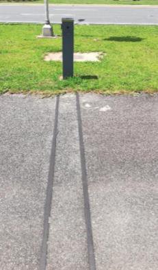
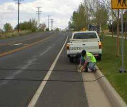
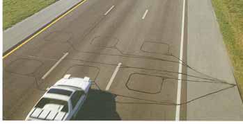
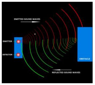
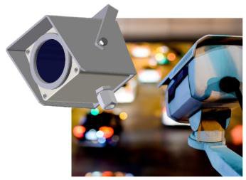
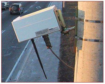
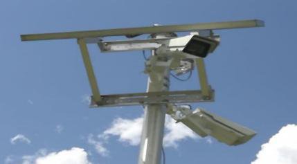
Ultrasound

Infrared (https://www.swarco.com/)

Microwave Radar

Video Camera

TDC1 Traffic Detector

• Advantages:
  • Suitable for gathering traffic data for longer period
  • Surveyors are not required
• Disadvantages:
  • Costly & sophisticated equipment are required
  • Need to check accuracy of devices

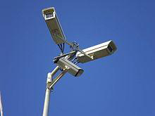
Video Taping Method

• Video camera placed at suitable elevated position to record the vehicle movement
• Recorded video processed at office later

• Advantages:
  • Less field Surveyors are required
  • Records are permanent and can be reviewed any time later
  • Opportunity to obtain wide range of data
• Disadvantages:
  • Costly video equipment are required
  • Additional office work is required

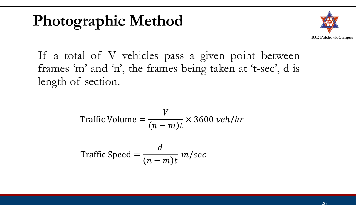
Photographic Method

• Photographs are taken at fixed intervals of time (e.g. 1 sec/ frame) on a special camera.

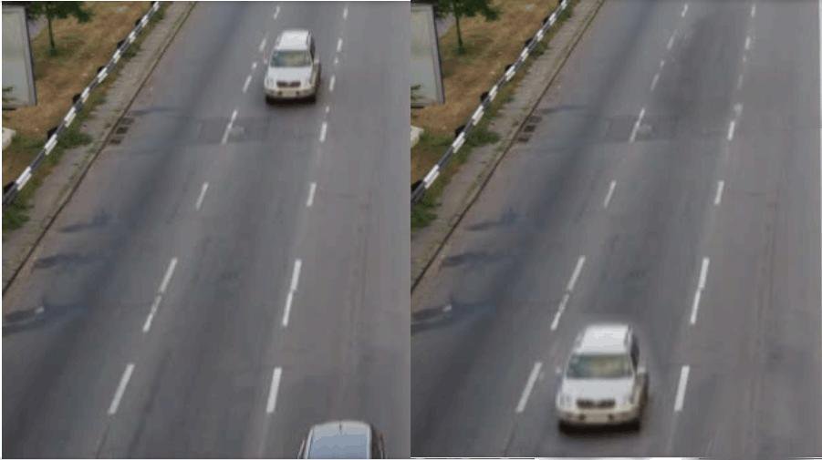
• Passage of vehicle is traced with reference to time.

Moving Observer (Floating Car) Technique20822076

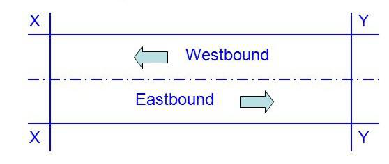
• A test vehicle is driven over a given section at the average speed of the stream
• A group of observers record the various details (Check in speed and delay study)

Traffic Volumes and Their Uses

• Daily volumes
• Hourly volumes
• Sub hourly volumes
• Cordon volume counts
• Intersection counts

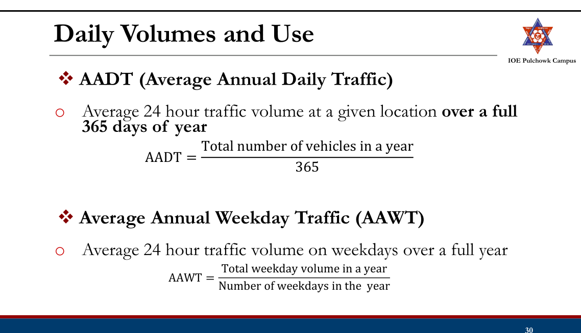
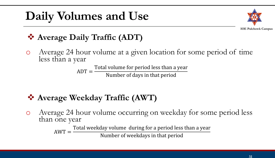
Daily Volumes and Use

• Common time interval for volume is day
• Used for highway planning and general observations of trends
• Traffic volume projections

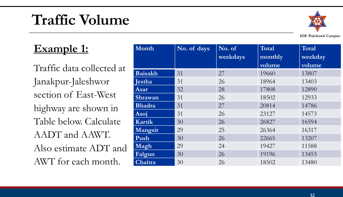
Traffic Volume

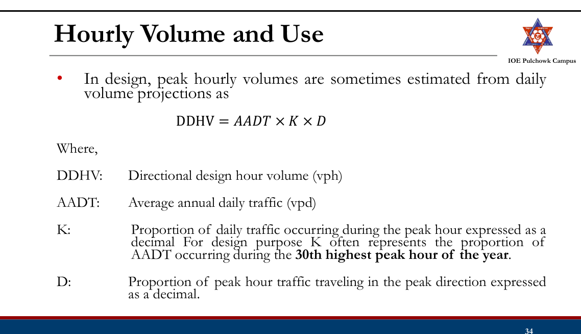
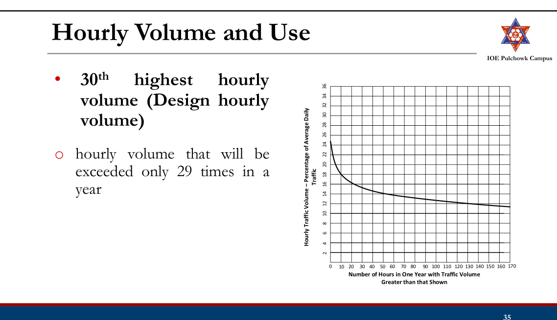
Hourly Volume and Use

• The single hour of the day that has the highest hourly volume is referred to as the peak hour and the corresponding hourly volume is peak hourly volume.
• Peak hour volume in peak direction of flow is of greatest interest to traffic engineers in design or operational analysis.

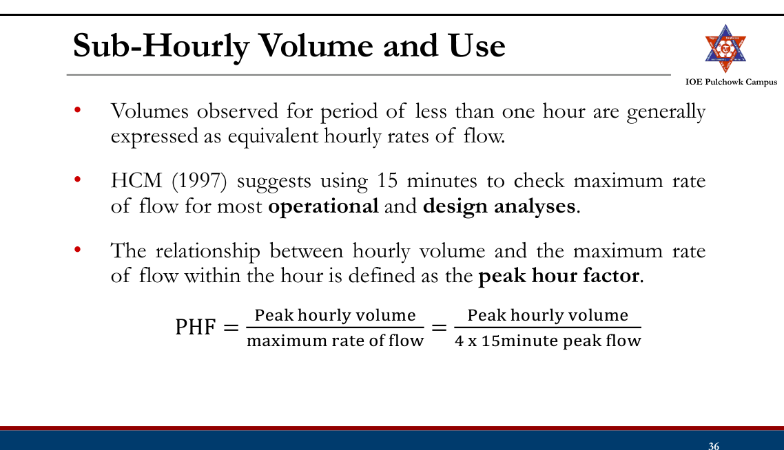
Sub-Hourly Volume and Use2080

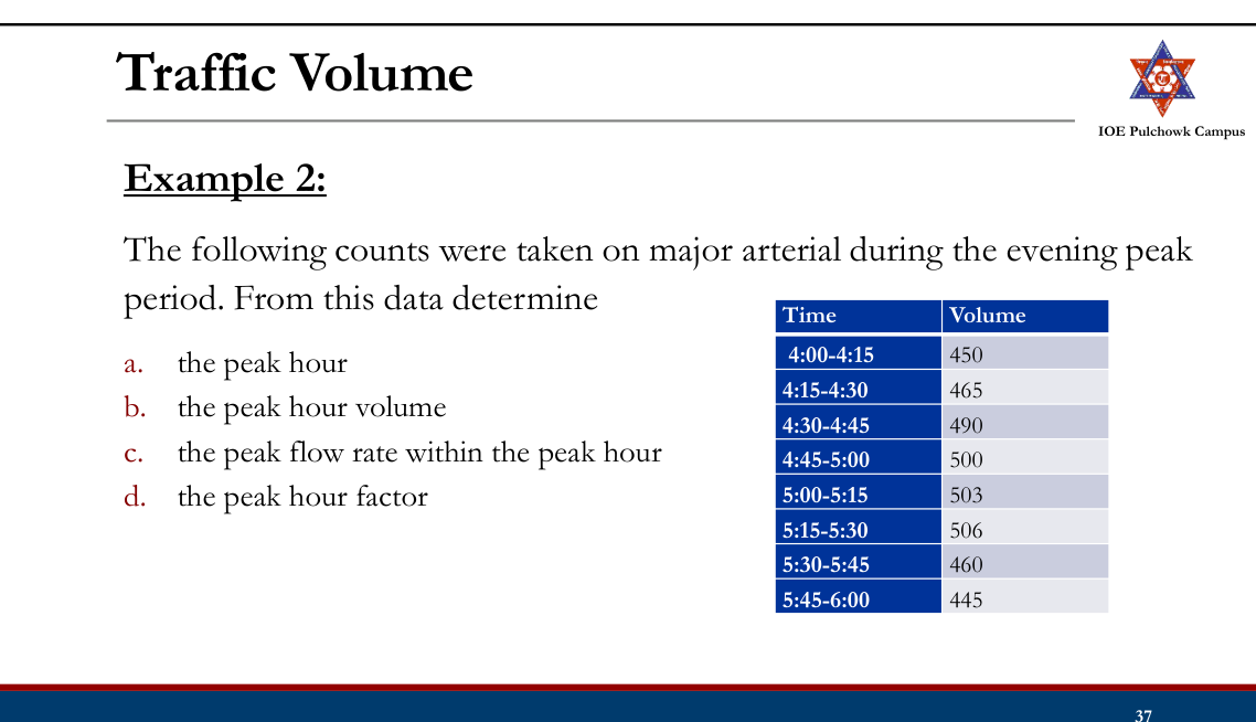
Traffic Volume

Cordon Volume Count and Intersection Count

• Cordon Volume Count:
• Accumulation of vehicles and/or persons within the cordon boundary (total of all counts entering and leaving the area by time period)
• Useful to estimate street capacity, parking needs etc. in similar land use type
• Intersection Count:
• At intersections, turning movements
• Useful for planning, signal timings, channelization and other control measures

Presentation of Traffic Volume Data

• Average Traffic Volumes
• Expressed in AADT or ADT, helps in deciding the relative importance of a route
• Normally expressed in PCUs.

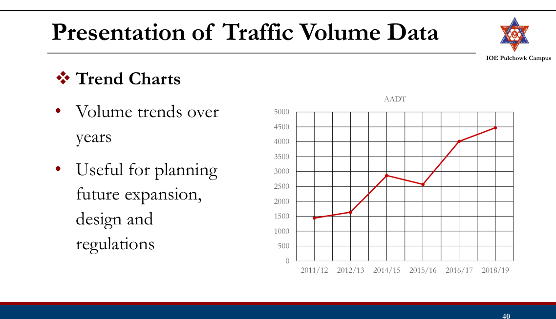
• Variation Charts

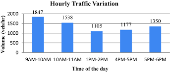
• Shows hourly, daily and seasonal variation
• Helpful for planning facilities and regulations needed during peak traffic period

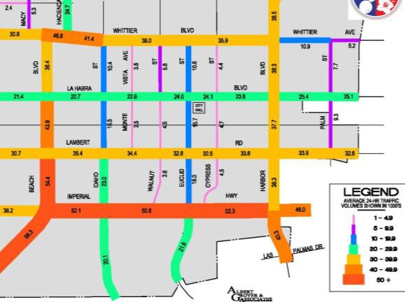
• Traffic Flow Map
• Shows volume along various routes by using bands proportional to traffic volume carried
• Help to visualize the traffic volume distribution at a glance

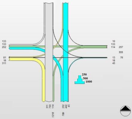
• Traffic Flow Diagram

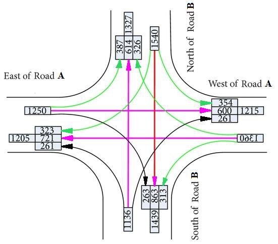
• Graphic representation of the traffic volume and directions of traffic movements through intersection

Poisson Distribution20812076

• Many traffic events such as vehicle arrival, crash occurrence are random processes
  • The events occurs continuously and are measured in terms of an average rate of occurrence over an interval (time/space)
  • The occurrence of events are independent
• Poisson (counting) distribution often used for modeling traffic phenomenon.

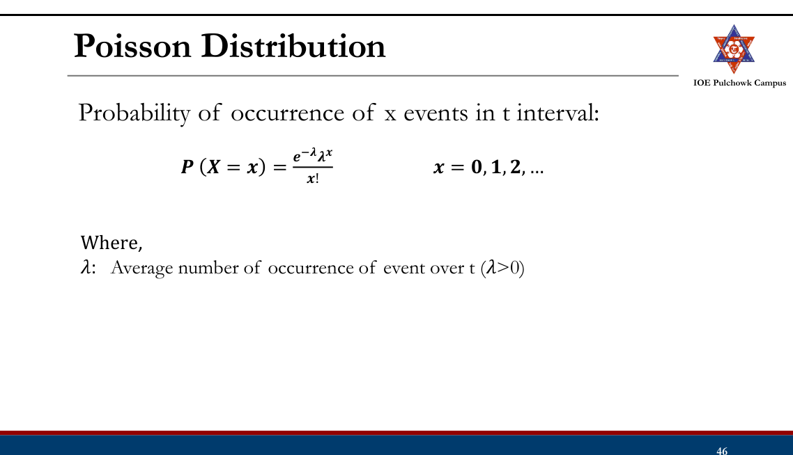
Numerical Example: The hourly flow rate in a road section is 120 veh/hr. Use Poisson distribution to model vehicle arrival at this road for 1 min time interval.

Tasks

• Review need and type of traffic studies
• Review volume studies: need, methods
• Review various traffic volumes and uses
• Review ways to present traffic volume data
• Review Poisson distribution

1.2 Traffic Speed and Delay Studies

Review

• Traffic studies
• Traffic volume studies Need, counting periods, methods
• Traffic volumes and uses
• Presentation of traffic volume data
• Poisson distribution

Speed Studies

• Speed is the rate of traffic movement
• Speed study is determination of the rate of traffic movement under specific conditions and for specific purpose

Types of Speed

• Spot Speed
• Average Speed (Time Mean Speed and Space Mean Speed)
• Running Speed
• Journey (Travel) Speed

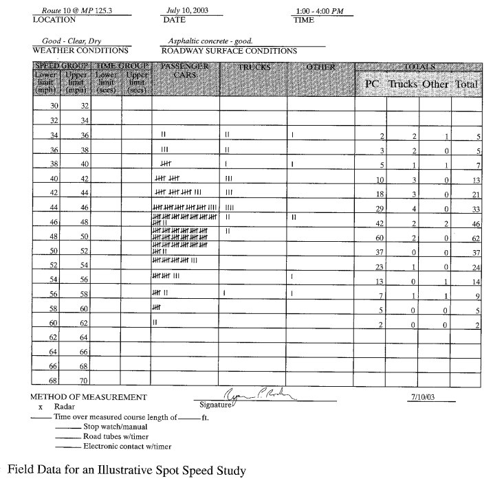
Spot Speed

• Instantaneous speed of vehicle at a specified location
• Uses:
  • To determine speed trend
  • Traffic capacity studies
  • Traffic operation and control
  • Geometric design of road
  • Crash studies
  • Before and after studies
  • Research studies

Average Speed

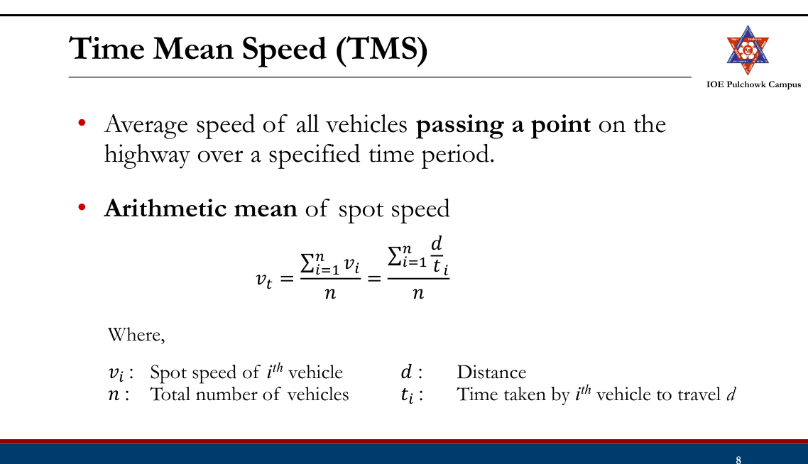
• Average of spot speed of all vehicles passing a given point on the highway
• It can be:
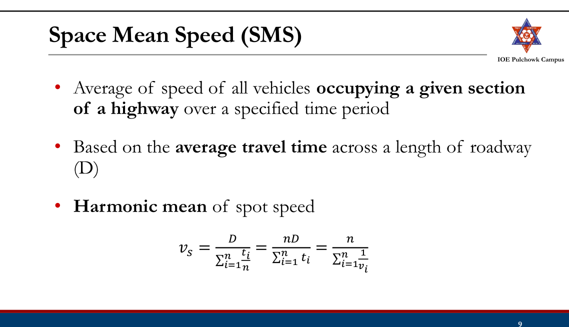
  • Space Mean Speed
  • Time Mean Speed

Time Mean Speed (TMS)

Space Mean Speed (SMS)20752066

Relationship Between SMS &TMS

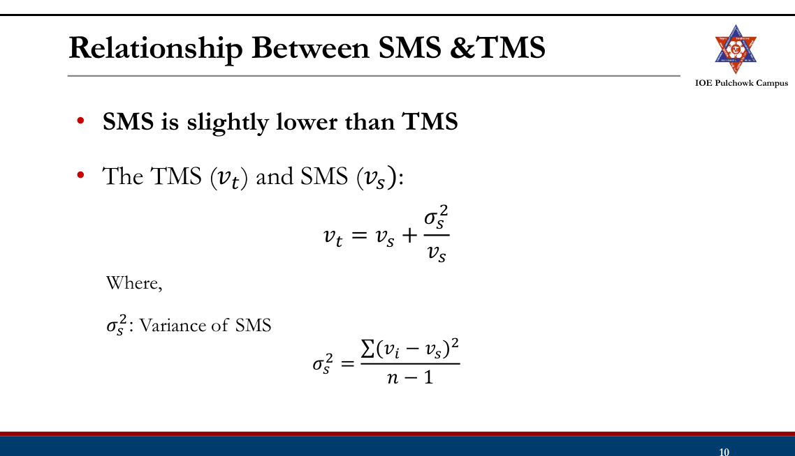
SMS & TMS

Numerical Example: Travel time (in second) measured for vehicles traversing 300m segment of a feeder road are 20.6, 21.7, 19.8, 20.3, 22.5, 18.5, 19.0, and 21.4. Determine the time mean speed and space mean speed of these vehicles.

Running Speed

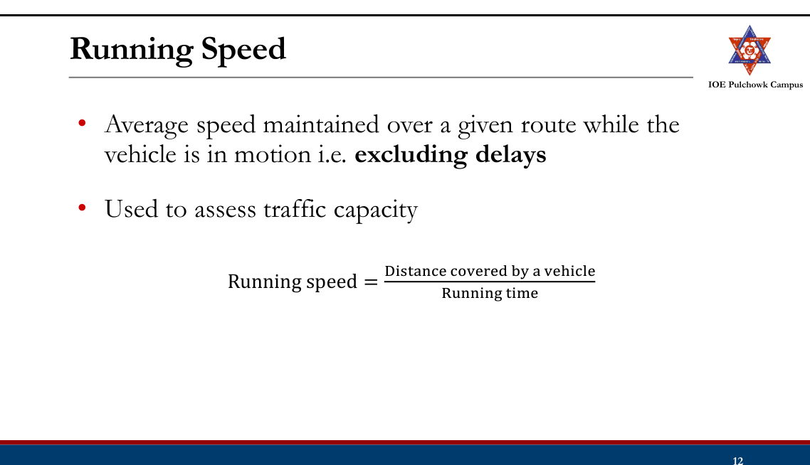
Journey (Travel) Speed

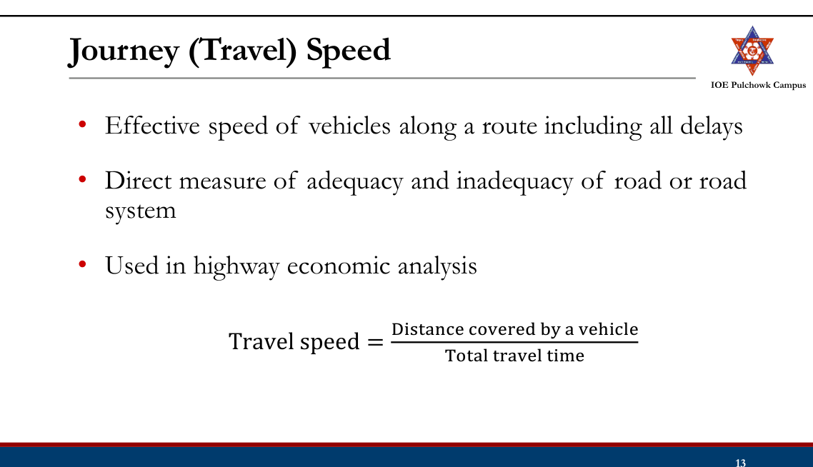
Methods of Spot Speed Measurement2081

• Manual
• Stop Watch (Direct) Method
• Enoscope Method
• Automatic
• Road Detectors (Pneumatic tube, Induction Loop)
• Radar meters
• Others
• Photographic, Videographic

Location

• If possible straight, level and open sections of highways should be selected
• Recommended base lengths:
  • Speed <40kmph: 27m
  • Speed 40 to 65kmph: 54m
  • Speed >65kmph: 81m

Sample Selection

• Random
• Representative (type, composition etc.)
• Free-flowing vehicles only
• At least 100 vehicles for 1 hour

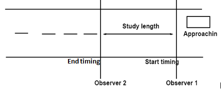
Stop Watch (Direct) Method

• Two reference points are marked on the pavement at a suitable distance apart.
• Single or two observers can be used to measure time

• Advantage:
  • Simple, easy and inexpensive
• Disadvantage:
  • Human errors
  • Parallax errors

Enoscope Method

• L-shaped box, open at both ends ,with a mirror set at 45 ˚ to the arms of the instrument.
• Measurement with two or one Enoscopes:

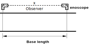
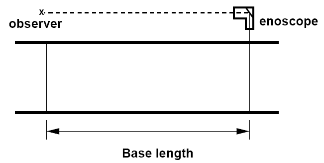
• Advantage:
  • Simple
  • Eliminates parallax error.
  • Equipment is of low cost and can set up easily
• Disadvantage:
  • Human errors
  • Not suitable for heavy multilane traffic

Pneumatic Tube Detector

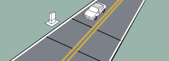
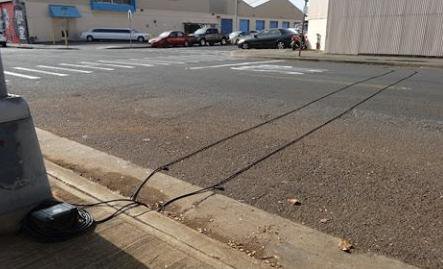
• Pneumatic tubes laid across the carriageway at the two reference point.
• When a vehicle passes over them, air impulses are sent to an electromagnetically controlled device.
• Time elapsed between first impulse and second impulse is recorded as speed.

• Advantage:
  • Human errors are eliminated
  • Accurate
• Disadvantage:
  • May affect driver behavior,
  • May disrupt traffic

Inductive Loop Detector

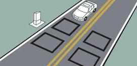
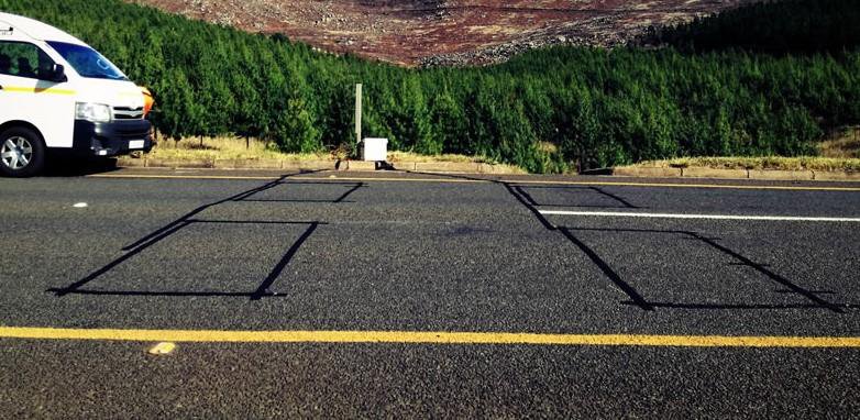
• A rectangular wire loop buried under the roadway surface, supplied with electromagnetic field
• A disturbance in the electrical field is created when a motor vehicle passes across it.
• Time difference between two loop is noted as speed.

Radar Meter

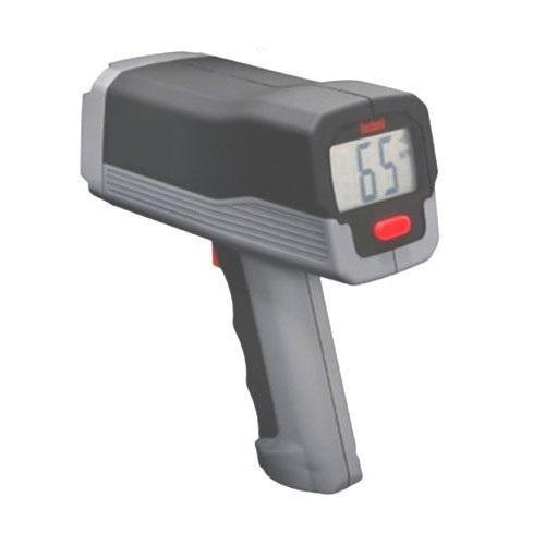
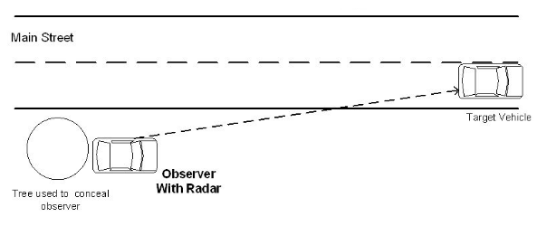
• Speed is proportional to change in frequency between the Radio wave transmitted and the radio wave received back.
• Instrument is setup near the edge of road at a height of 1m and target the vehicle, which gives speed directly.
• Hand held radar units (radar guns) are also used.
• Conceal the operation



• Cosine correction: Minimize cosine error by keeping angle <7o on freeways, <9o on urban streets

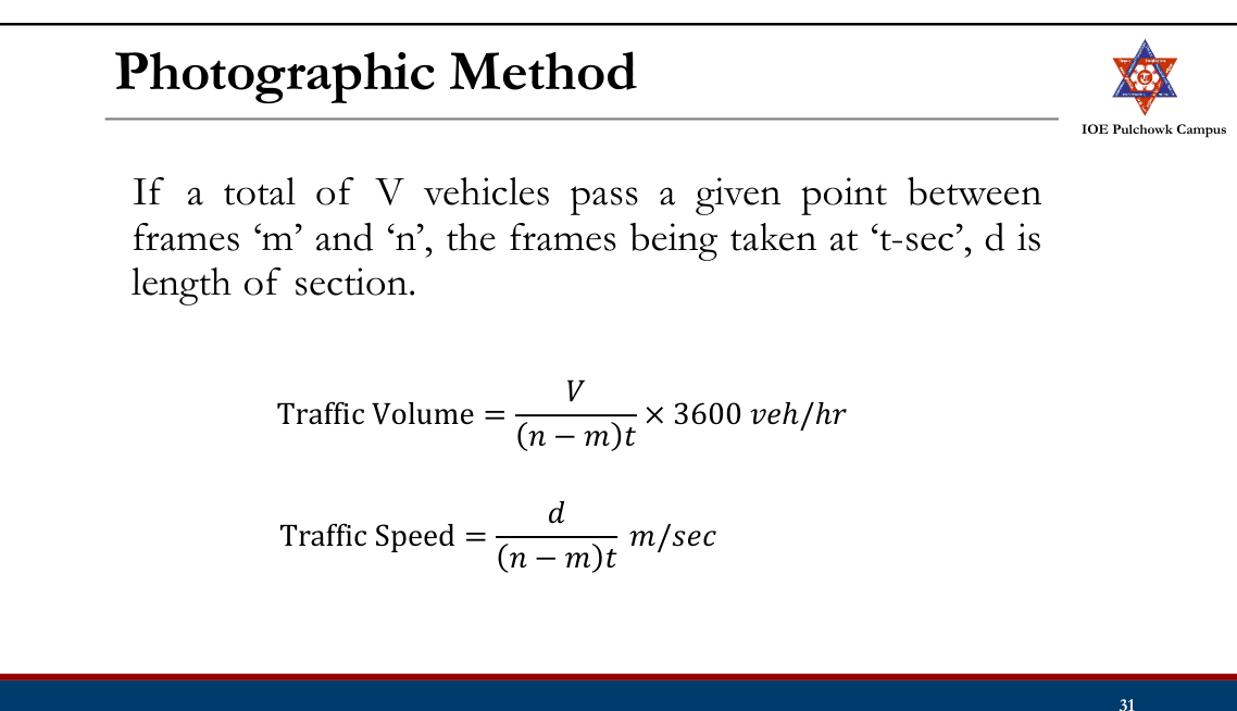
Photographic Method

• Photographs are taken at fixed intervals of time (e.g. 1 sec/ frame) on a special camera.

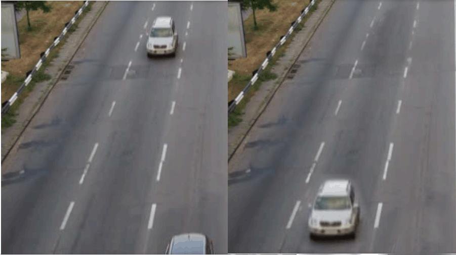
• Passage of vehicle is traced with reference to time.

Video graphic Method

• Video camera placed at suitable elevated position to record the vehicle movement

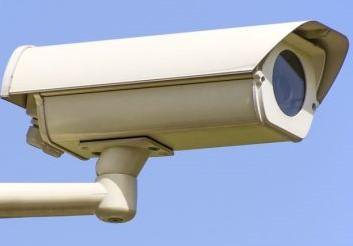
• Recorded video processed at office later to obtain speed
• Useful to determine speed of vehicles in crowded streets

Presentation and Analysis of Spot Speed Data

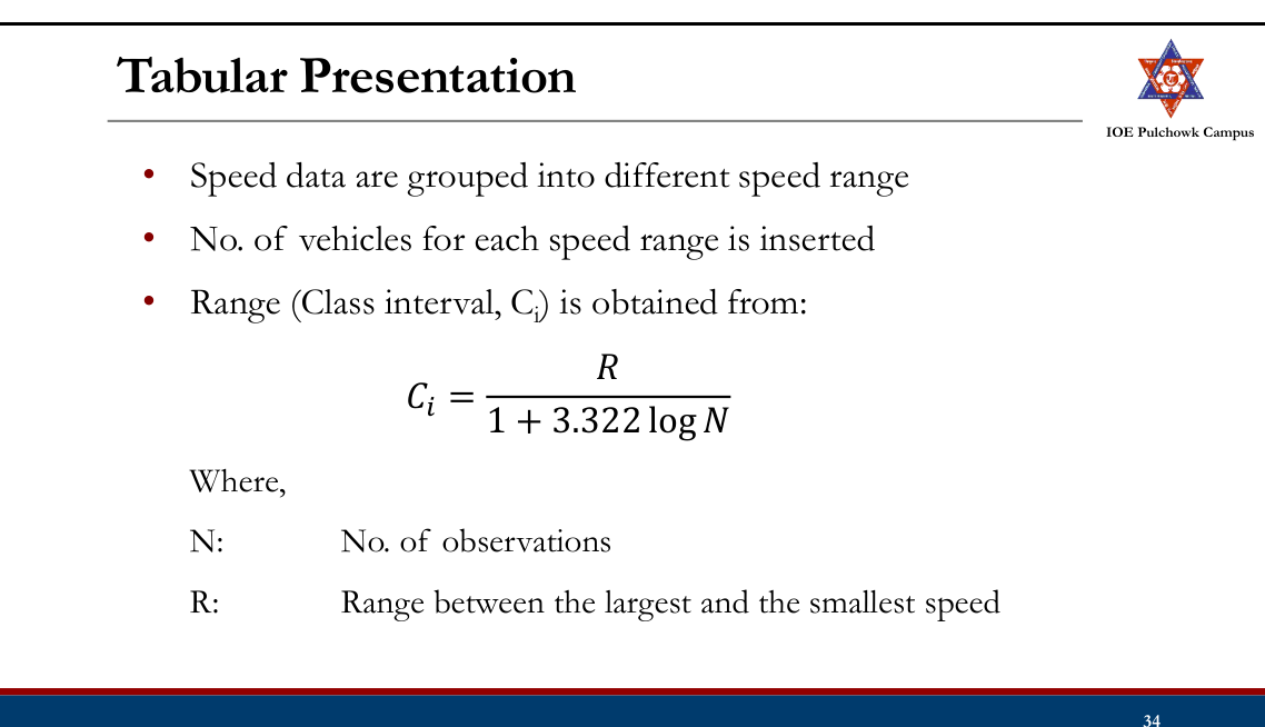
• Tabular Presentation
• Statistical Analysis
• Graphical Presentation

Tabular Presentation

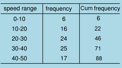
Statistical Analysis

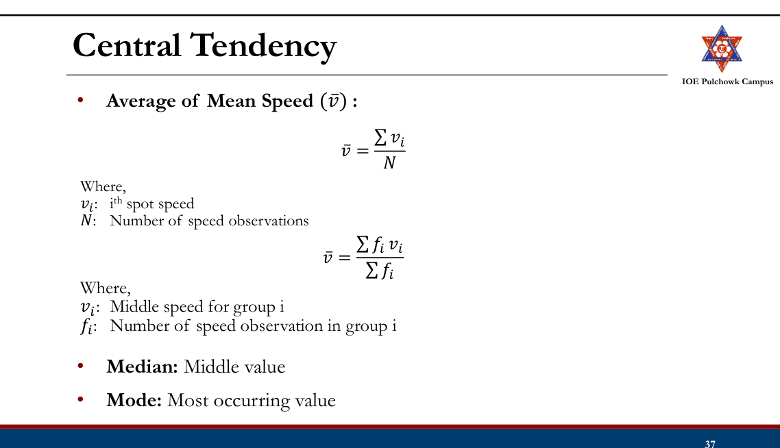
• Measures of central tendency
  • Mean, Median, Mode
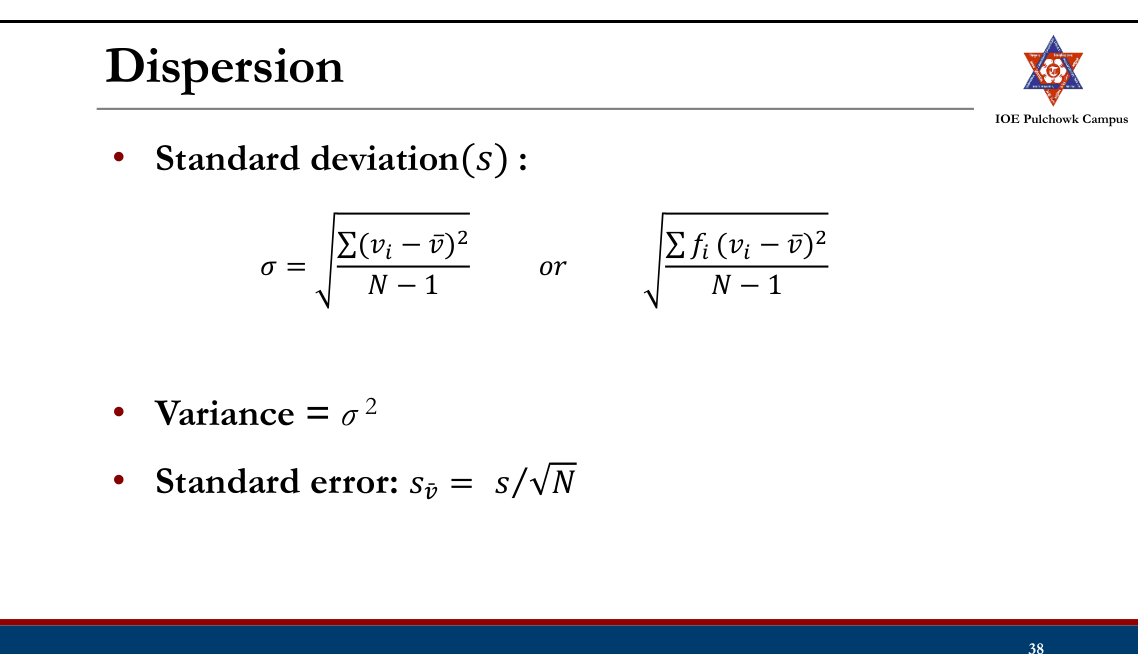
• Measures of dispersion
  • Standard Deviation, Standard Error
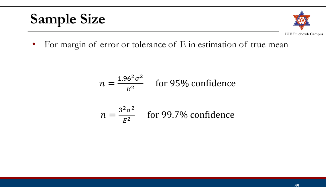
• Estimating sample sizes

Central Tendency

Dispersion

Sample Size

Graphical Presentation

• Frequency histogram
• Frequency curve
• Cumulative frequency curve

Histogram

• Graphical representation with x- axis as spot speed and y-axis as frequency

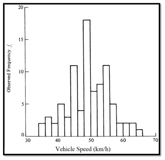
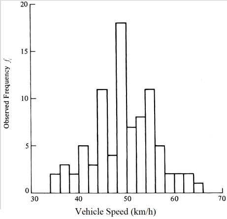
Frequency Curve

• Bell shaped curve obtained by a line joining mid points of histogram

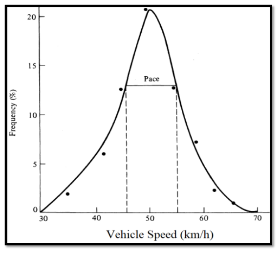
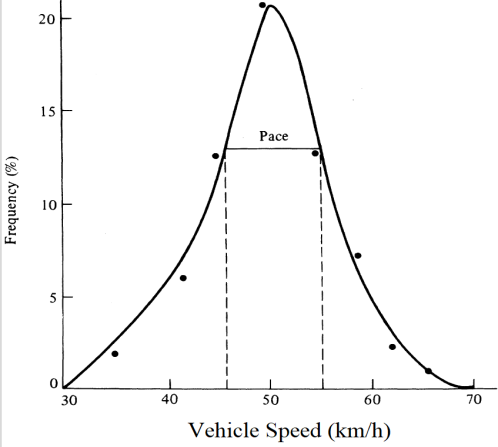
• Useful to check normality of data
• Modal speed: Drop a vertical line from the peak of the frequency curve
• Pace: 10Km/h increment in speed in which the highest % of drivers is observed

Cumulative Frequency Curve2074

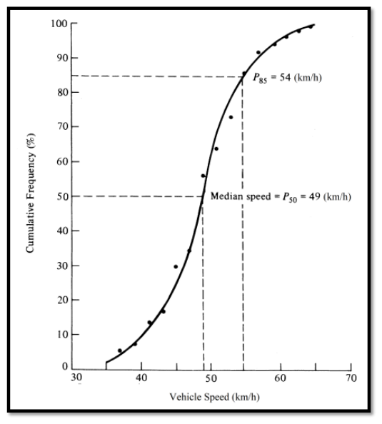
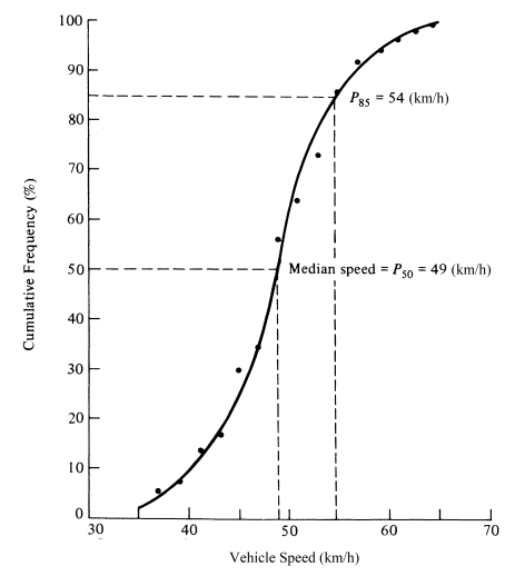
• Curve obtained by plotting the cumulative % against the upper limit of speed range
• Smooth S-curve is obtained

• Use:
  • 98% - Design speed
  • 85% - Upper speed limit
  • 50% - Median Speed
  • 15% - Lower speed limit

Spot Speed

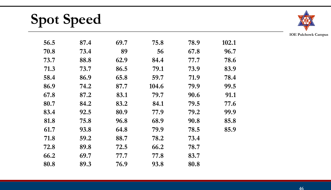
Numerical Example The data collected in kmph on 86 vehicles in a rural road during spot speed study is shown in table below. Develop the frequency histogram, frequency distribution, and

cumulative frequency of data and determine: i) Mean speed and space mean speed ii) Standard deviation iii) Median speed iv) Modal speed v) Pace vi) Speed limit for regulation vii) Speed to check geometric design viii) Lower speed limit

Normal Distribution to Spot Speed2071

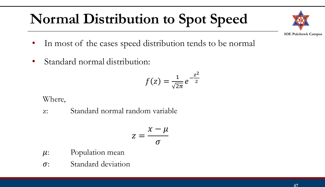
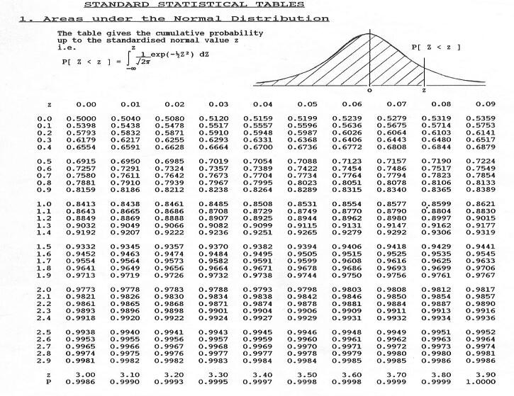
Numerical Example: A spot speed at particular location are normally distributed with a mean of 51.7 kmph, standard deviation of 8.3kmph. What is the probability that the speed exceeds a) 65kmph. b) Speed lies between 40-70kmph. c) What is the 85th percentile speed?

Delay

• Time lost during the travel due to disruption of traffic movement
• Measured as the time difference between actual travel time and free-flow travel time
• Types:
  • Fixed: At intersections due to traffic signals
  • Operational: By interference of traffic movements e.g. turning movements and internal friction in the traffic stream e.g. high volume

Speed and Delay Study

• Determine running speeds, overall speeds, fluctuations in speeds and delay between two stations of a road spaced far apart
• Uses:
  • To detect spots of congestion and causes
  • To find travel times in specific links
  • To determine level of service
  • For benefit cost analysis
  • For before after studies

Methods of Speed and Delay Study

• License Plate Observations
• Observation from Vantage Point
• Photographic and Video Survey Method
• Interview Method
• Moving Observer (Floating Car) Technique

License Plate Observations

• Observers at entrance and exit record license plate number and time of vehicles

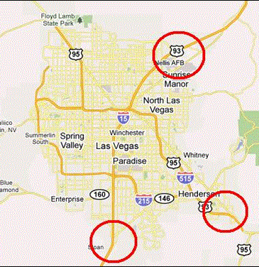
• The license plate number recordings are matched and the difference in time is the travel time of the vehicle
• Average of travel times of vehicles (at least 50 matched sample) is the average traveling time on the test section

Observation from Vantage Point

• Average travel time, number of delays, duration and causes are recorded through observations of vehicles from an elevated point
• Suitable only for short section

Photographic and Video Survey Method

• Same as in Volume and Speed study
• Useful for short stretch of section

Interview Method

• Road users of of the study site are interviewed regarding their travel times, experience of delays.
• Used when large amount of information is needed in short time
• Requires cooperation of the people

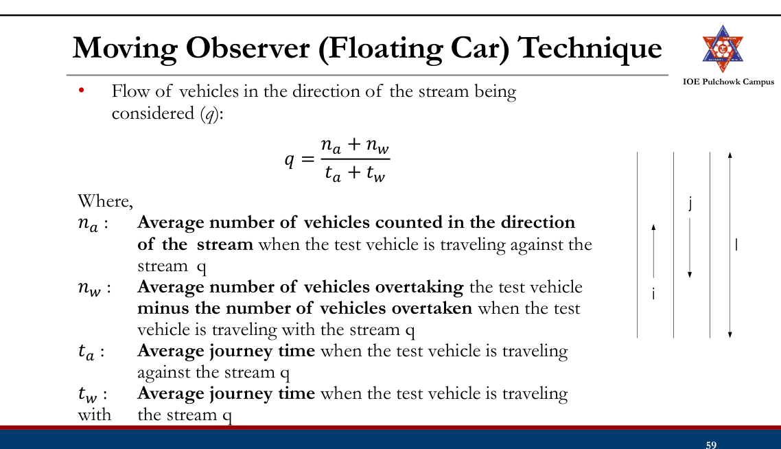
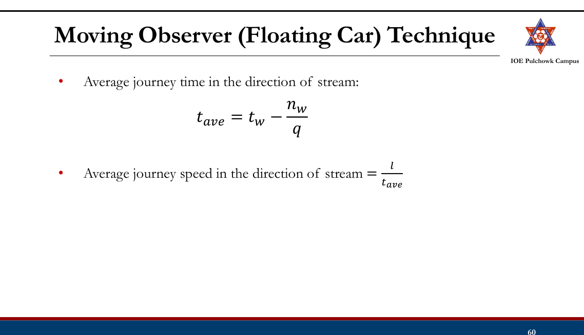
Moving Observer (Floating Car) Technique2072

• A test vehicle makes a series of runs on a road section on both directions at approximately the average speed of the stream. j l
• Minimum 6 runs on each direction i

• A group of observers make record of various

details:

• Journey Observer: Start and end time of journey; time, location and cause of delays
  • Opposing Counter: No. of vehicles travelling in the opposite direction in each trip
  • Tally Counter: No. of vehicles overtaking the test vehicle and no. of vehicles overtaken by the test vehicle in each trip

Numerical Example: The consolidated data collected from speed and delay studies by floating car method on a stretch of urban road of length 3.5 km running North-South are given below. Determine the average values of volume, journey speed and running speed of the traffic stream along either direction. Trip no. Direction of trip Journey time Total stopped delay No. of vehicles Overtaking Overtaken From opposite direction N-S S-N N-S S-N N-S S-N N-S S-N min sec min sec

Tasks

• Review spot speed, average speed (TMS & SMS), journey speed, running speed
• Review methods of speed measurement (stop watch, enoscope, pneumatic tube, inductive loop, radar meter, photographic and video graphic method
• Review tabular and graphical presentation and statistical analysis of spot speed data
• Review normal distribution to spot speed
• Review speed and delay study and its uses
• Review methods of speed and delay study
• Review moving observers or floating car technique for speed and delay study

1.3 Origin and Destination Study

Review

• Spot speed, TMS, SMS, running speed, travel/journey speed
• Methods of spot speed measurement
• Presentation and analysis of spot speed data
• Normal distribution for spot speed analysis
• Speed and delay study and its uses
• Methods of speed and delay study
• Moving observers or floating car technique

Origin and Destination (O-D) Study

• Origin: Place where the trip begins
• Destination: Place where the trip ends
• O-D study reveals:
  • Actual/desired direction of travel, routes and length of trip
  • Amount of travel between various locations or within particular location
  • Relationship between amount and type of travel and the traffic generating factors

Uses of O-D Study2071

• To judge the adequacy of existing routes and plan transportation system (new network of roads, mass transit facilities including plans for operation)
• To locate major routes along the desire lines
• To establish by pass route
• To locate terminals and plan terminal facilities
• To locate new bridges as per traffic demands
• To establish design standards

O-D Data

• Area under O-D survey is divided into various zones uniform in characteristics and bounded by natural or artificial boundaries like river, lakes, rail, roads etc. z1 z2 z3
• Information collected:
  • Number of vehicular trips, their O-D origin and destination in each zone under study (O-D matrix)

• Additional information collected:
  • Land use patterns, household characteristics
  • Trip details: Purpose of trip, time and mode of trip, number of passengers in each vehicle, intermediate stops and reasons etc.

Methods of O-D Survey

• Road Side Interview Method
• Home-Interview Method
• Work Spot Interview Method
• License Plate Method
• Post card Method
• Tag on Vehicle Method
• Commercial Vehicle Survey

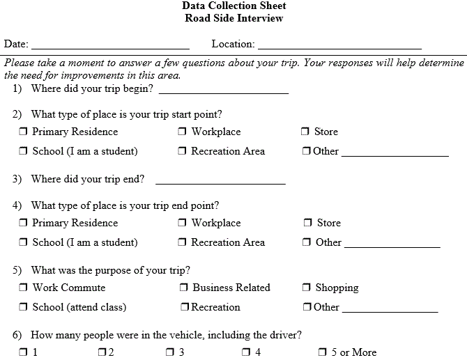
Road Side Interview Method

• The vehicles are stopped at the interview stations by a group of surveyor
• Drivers are questioned using prescribed questionnaire about
  • Origin and Destination
  • Trip time, purpose, frequency

• Sampling:
  • Simply next vehicle after interviewing one;
  • A fixed number of vehicles (eg. 3 out of 12 vehicles);
  • % by time (e.g. all vehicles in every half hour)

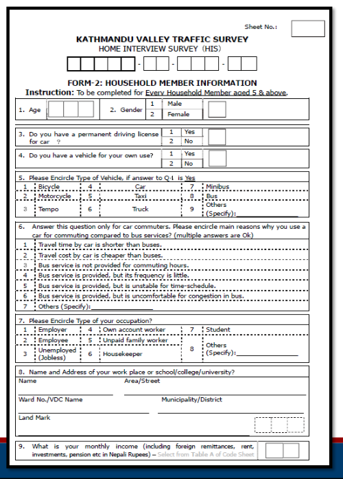
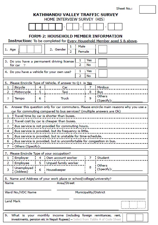
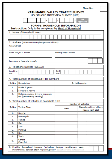
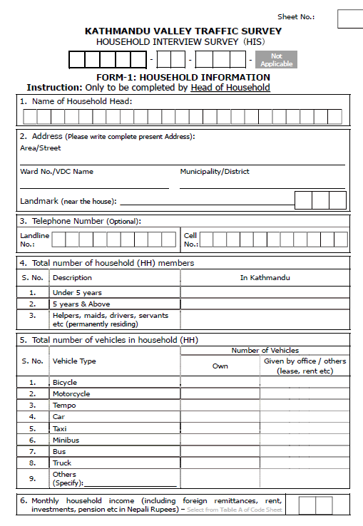
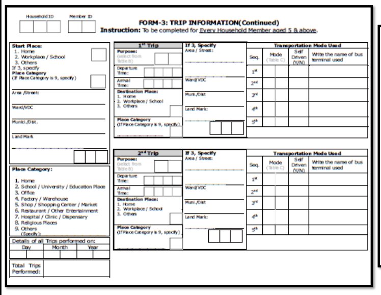
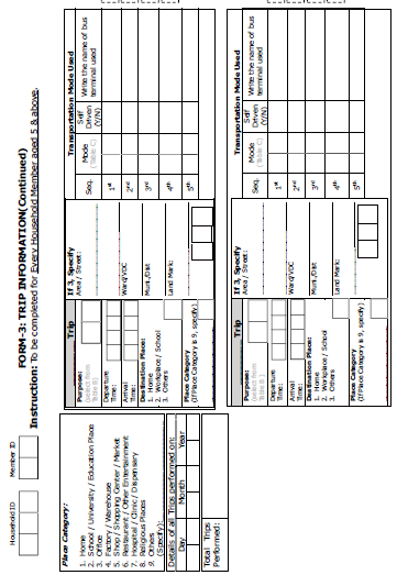
Home Interview Method

• A representative sample (about 10% of population) is selected
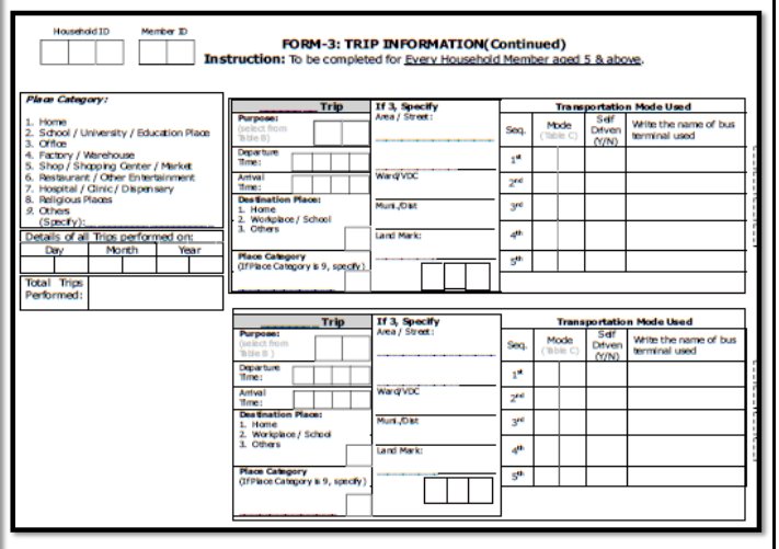
• Detailed information on household characteristics and travel information are collected through interviews and questionnaire forms.
• Suitable to obtain comprehensive details
• Useful for planning road network and particularly mass transportation facilities

• Information collected:
  • Household information: Household size, income, vehicle ownership, driving license etc.
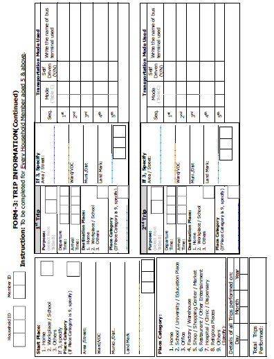
  • Household travel data: O-D of all trips, start and finish times of journeys, journey purpose, mode of travel, number of occupants, public transport route and cost, details of parking utilized etc.

Work Spot Interview Method

• Work spot like office, factories, institutions can be chosen for survey
• Origin-destination, parking requirement and other information are collected

License Plate Method

• A number of survey points are fixed.
• Registration number and class of each vehicle entering or leaving an area at survey points located on the cordon line are noted.
• Information obtained from all the survey points are tallied and origin destination data are obtained.
• Data collection does not interrupt traffic.
• Large number of stations and large number of study personnel are required.

Post Card Method

• A questionnaire with required information is printed on post card.
• Pre-paid post cards are handed over to each of the drivers at the survey points
• The road users are requested to answer the questions and return by post.
• Simple and little interference to traffic
• Return rate is less (30% is typical)

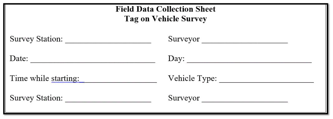
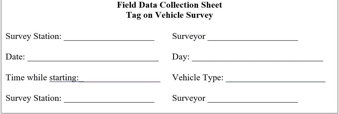
Tag on Vehicle Method

• A tag or sticker of particular shape and color is stuck on the windscreen of each vehicle entering the survey area.
• The place of entry and time is marked.
• The tag is taken back as it leaves the survey area and the time and station are recorded.

Commercial Vehicle Survey

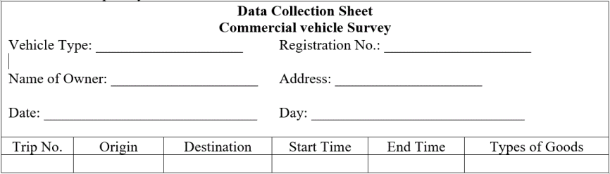
• Operators are contacted to obtain information on journeys made by commercial vehicles.
• Questionnaire are issued to drivers with a request to record their trips.

Presentation of O-D Data

• OD Table (Matrix)
• Desire Lines

O-D Table

• Horizontal axis of the matrix represents the Destination zone
• Vertical axis represents the origin zone
• The number of trips are entered in the cells of matrix Destination zone T11 T12 T13 T21 T22 T23 T31 T32 T33 Origin zone

Desire Lines

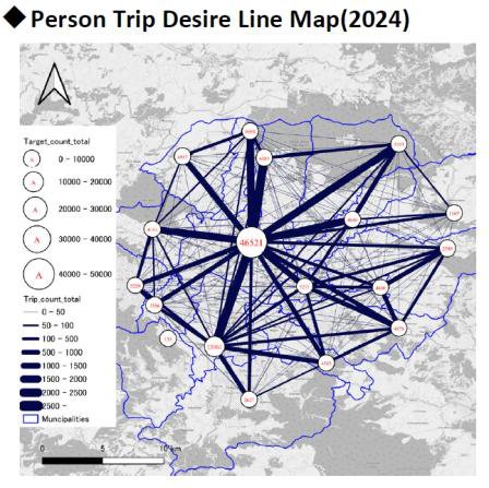
• They are straight lines connecting the centroids of the two zones
• Width of line is drawn to a suitable scale to represent the nos. in both direction z1 z2 z3 JICA (2024) Kathmandu Valley Urban Transport System Master Plan

Presentation of O-D Data

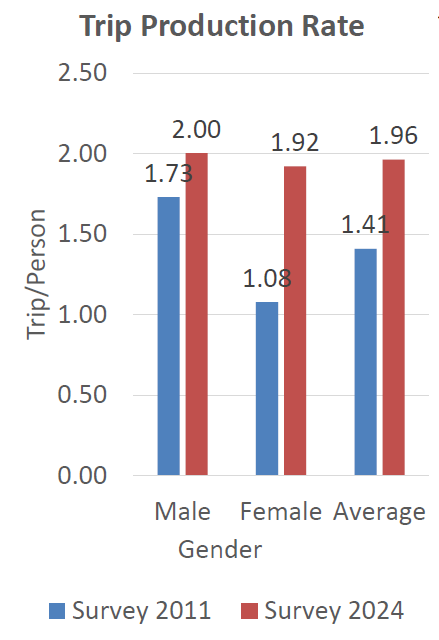
Valley Urban Transport System Master Plan:

• Household Interview Survey of 21372 households, around 2.5% of population of 18 municipalities in KV
• 222 zones (each ward in the municipalities) JICA (2024) Kathmandu Valley Urban Transport System Master Plan

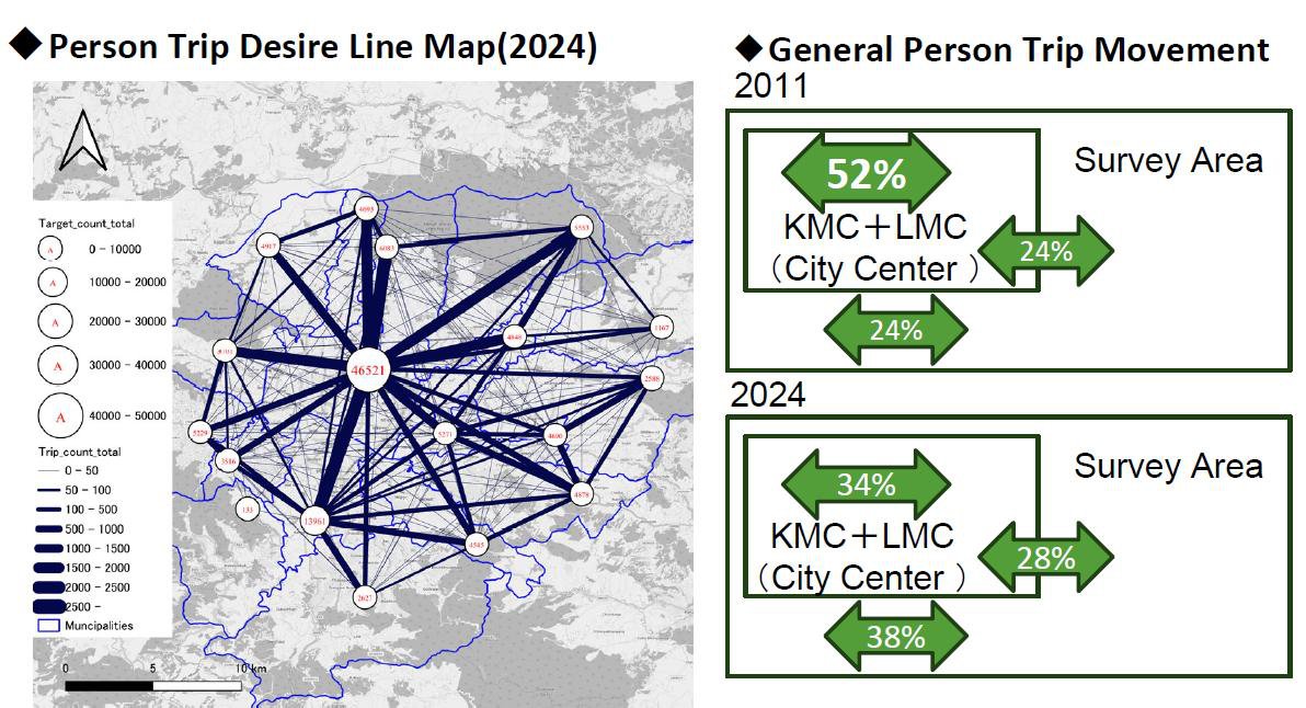
JICA (2024) Kathmandu Valley Urban Transport System Master Plan

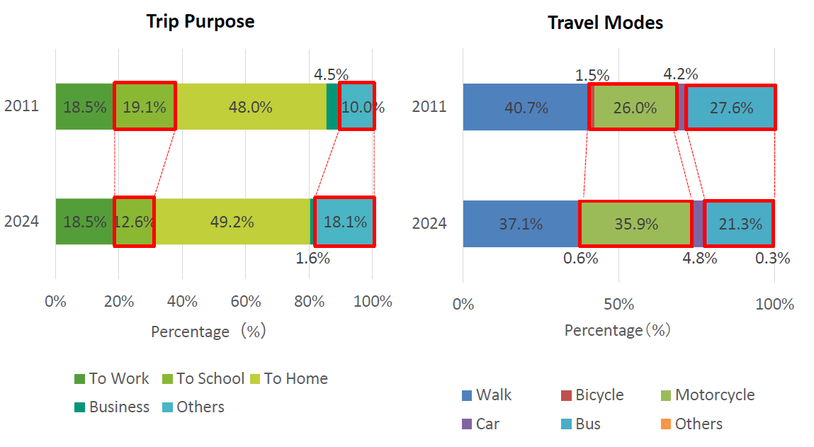
Shopping increased from 4 to 7.6%, Leisure/recreation increased from 1.8 to 5.5% JICA (2024) Kathmandu Valley Urban Transport System Master Plan

Tasks

• Review OD survey and its uses
• Review methods of OD survey
• Review presentation of OD survey data

1.4 Basic Traffic Flow Parameters

Review

• OD survey and uses
• Methods of OD survey
• Presentation of OD data

Basic Traffic Flow Parameters

• Traffic flow refers to the movement of vehicles through space and time.
• Traffic flow characteristics are affected by vehicle types, road users, and roadway and traffic conditions.
• Essential for the analysis, design, and operational management of traffic streams.

1. Flow (q): Number of vehicles/volume passing a fixed roadside point per unit time (vph)
2. Speed (v): Space mean speed of vehicles (kmph)
3. Density (k): Number of vehicles located in a given length of lane or roadway at a particular instant in time (vpkm)

The relation between speed, density, and flow is: 𝑞= 𝑘𝑉 (Fundamental relationship in traffic flow theory)

Other Traffic Flow Parameters

• Spacing/Space Headway (s):
• Distance between successive vehicles in a traffic stream as measured from front bumper to front bumper.

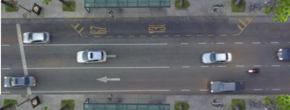
S1

S2 𝑘= 1 𝑠

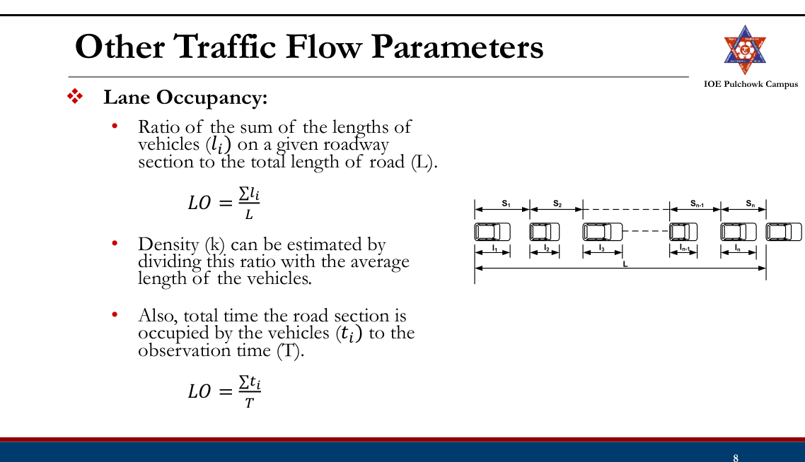
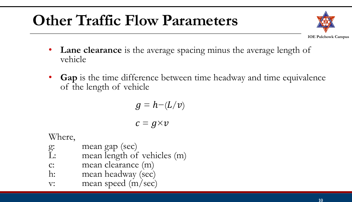
• Clearance and Gap:
• Correspond to spacing (m) and headway (sec). Clearance (m) L (m) Gap (sec) Spacing (m) or Headway (sec)

Time Space Diagram

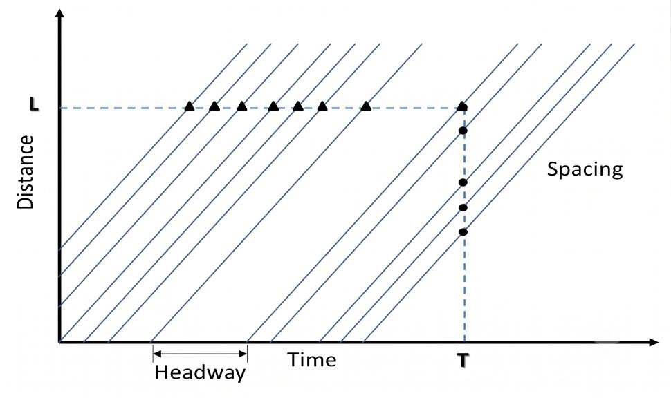
Basic Traffic Flow

Parameters

• Flow
• Density
• Speed
• Space headway
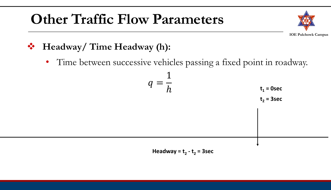
• Time headway

Traffic Flow Conditions

• Uninterrupted:
• It occurs at the facilities where there are no external factors such as traffic signal that cause periodic interruption to the traffic stream.
• Eg. Freeways, limited-access facilities, where there are no traffic signal, stop or yield signs, or surface intersections. It may also exist in long sections of rural highway between signalized intersections.
• Flow breakdown is due to internal factor only.

• Interrupted:
• It occurs at the facilities that have external devices that periodically interrupt traffic flow
• The principal device creating interrupted flow are the traffic signal, stop sign etc.
• Flow occurs in platoons.

Analysis of Speed, Flow and Density Relationship20812074

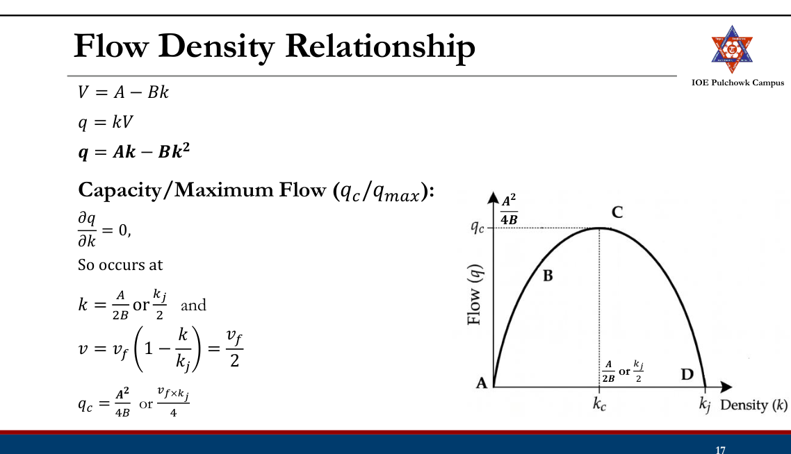
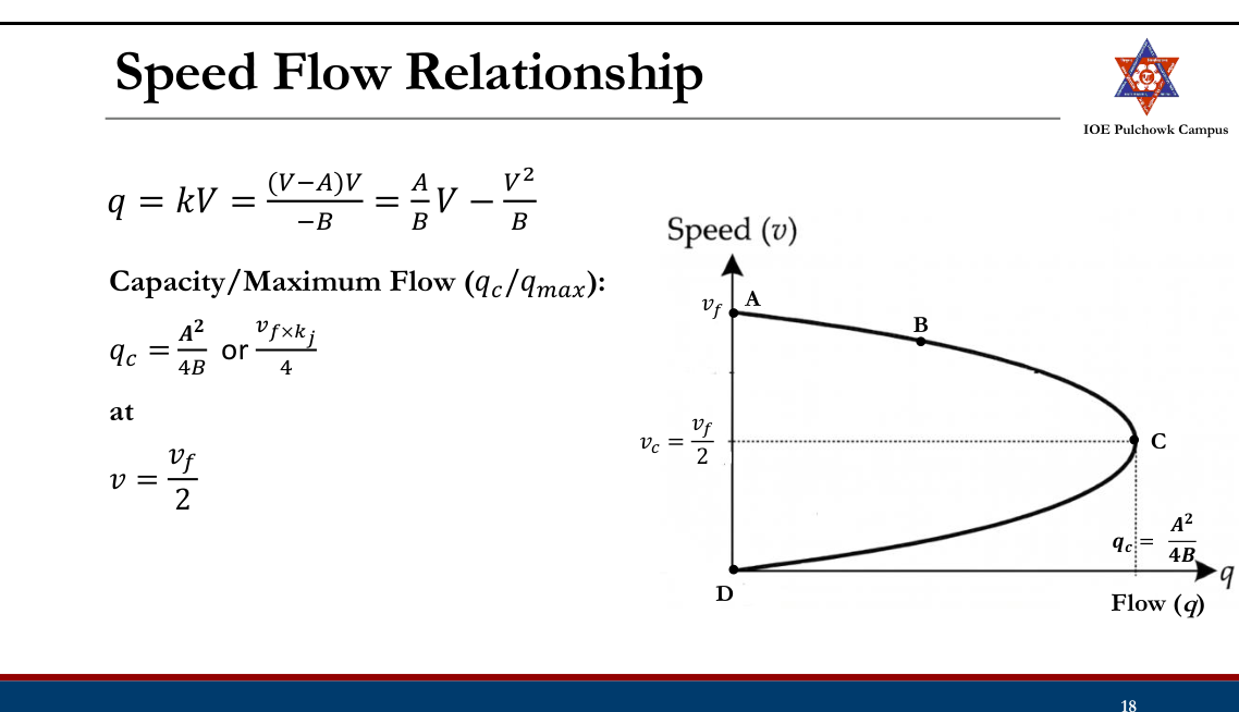
Uninterrupted traffic flow:

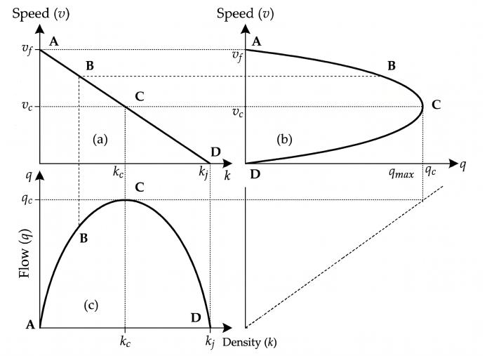
• Points A, B, to C: Normal Flow
• Points C to D: Forced flow

Speed Density Relationship20812072

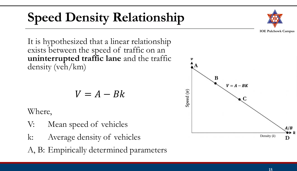
𝑣𝑓 :

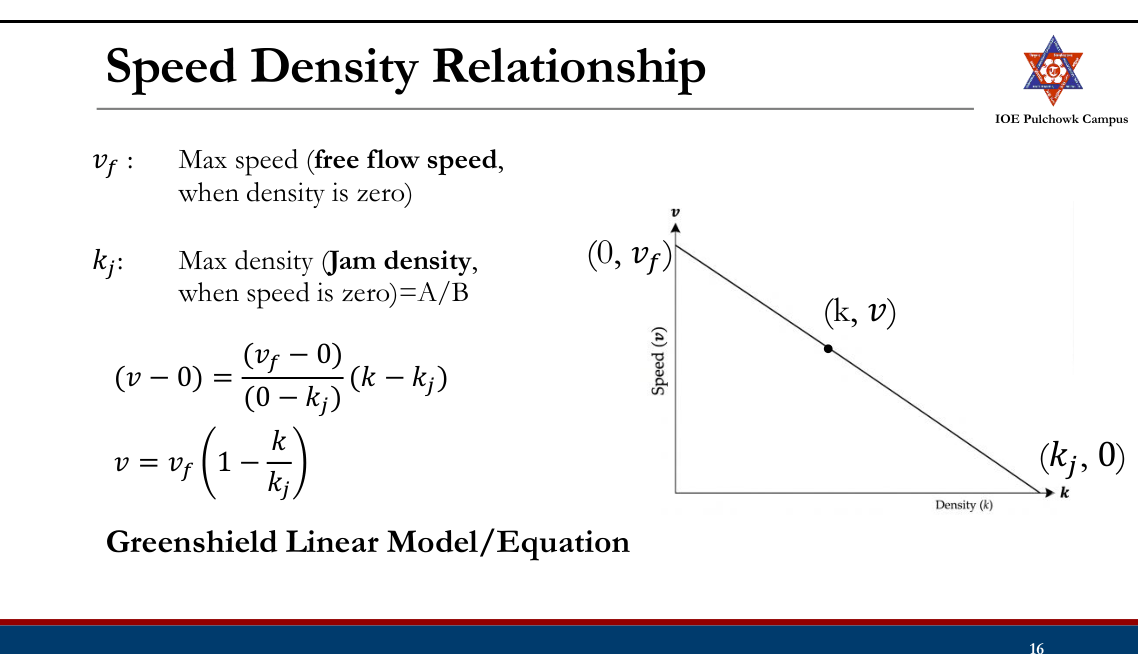
Flow Density Relationship

Speed Flow Relationship

Basic Traffic Flow Parameters

Example: A study of freeway flow at a particular site has resulted in a calibrated speed density relationship as follows: 𝑉 = 57.5(1 − 0.008𝐾). For this relationship, determine, (a) free flow speed (b) jam density (c) capacity and d) plot speed flow relationship and e) flow density relationship. What will be the speed and density value for highest level of service possible if the flow is 80% of the capacity flow? Calculate spacing, headway, gap and clearance when there is capacity flow if the length of vehicle is 6.1m.

1.5 Traffic Capacity and Level of Service

Traffic Capacity2080

• Maximum numbers of vehicles that a highway element can be expected to accommodate under a given set of condition.
• HCM defines the capacity of a facility as the maximum hourly rate at which persons or vehicles can be reasonably expected to traverse a point or uniform segment of a lane or roadway during a given time period under prevailing roadway and traffic conditions.
• Uses: Analysis, design and improvement of transport facilities

• Basic capacity
• Possible capacity
• Practical capacity

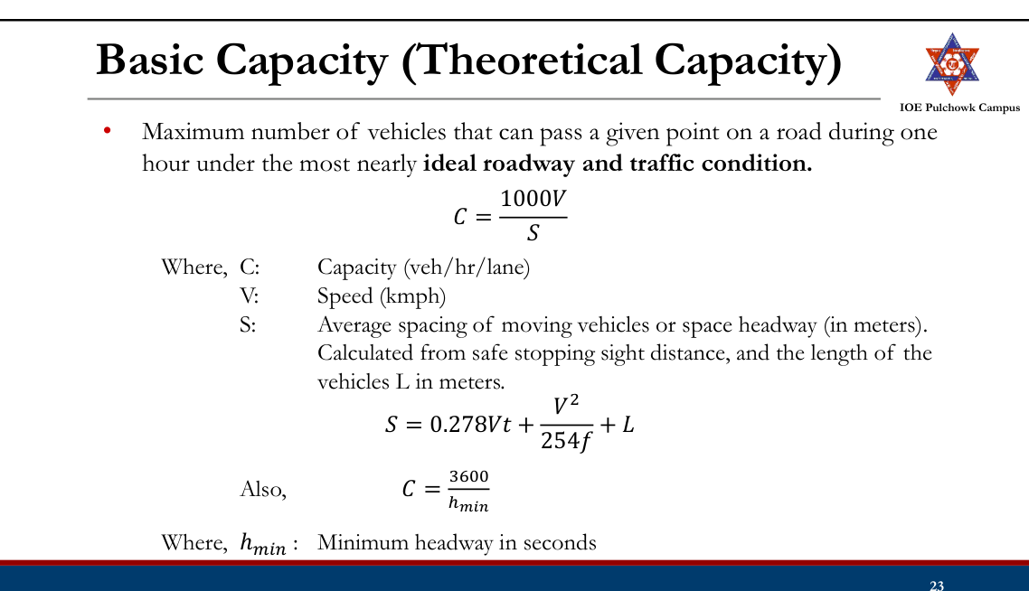
Basic Capacity (Theoretical Capacity)

Possible and Practical Capacities

Possible Capacity

• The maximum number of vehicles that can pass a given point on a lane or roadway during one hour, under the prevailing roadway and traffic conditions. Practical Capacity
• The maximum number of vehicles that can pass a given point in a lane or roadway during one hour, without the traffic density being so great as to cause unreasonable delay, hazard or restriction to the drivers' freedom to maneuver under prevailing roadway and traffic conditions.
• Also called ‘design capacity’.

Traffic Capacity

Example: Calculate the theoretical capacity of a traffic lane with one way traffic flow at a stream speed of 65 kmph. Assume coefficient of friction as 0.38, total reaction time as 0.68 sec and average length of vehicle as 6.1 m.

Capacity and Level of Service

• When traffic volume equals the capacity of a highway, operating conditions are poor, even under ideal roadway and traffic conditions.
• LOS is a qualitative measure describing operational conditions within a traffic stream.
• Depends on several factors.

Level of Service2080

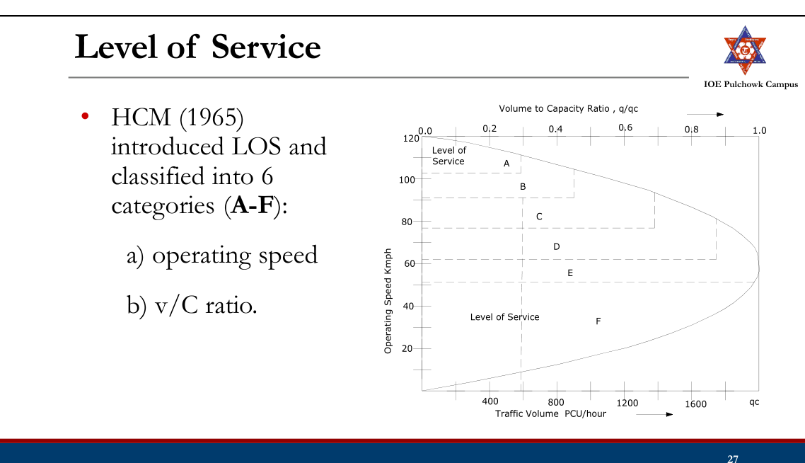
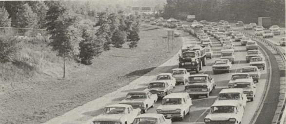
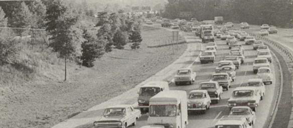
LOS A: LOS B: Free flow, free maneuver, average spacing 161m (528 ft), v/c ratio ≈ 0.3 Stable flow, reasonably free flow, maneuvering still easy, average spacing 100m (330 ft), v/c ratio ≈ 0.45

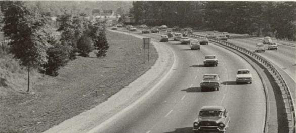
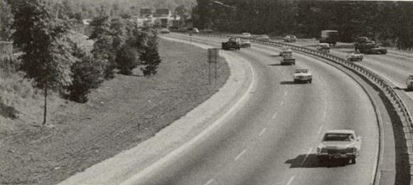
LOS C: LOS D: Stable flow, maneuverability noticeably restricted, satisfactory operating speed still maintained, average spacing 67m (220 ft), v/c ratio ≈ 0.7 Unstable flow, speed decline, maneuvering difficult and driver looks for gap, average spacing 50m (165 ft), v/c ratio ≈ 0.9

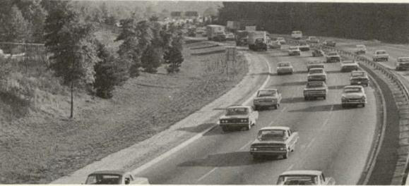
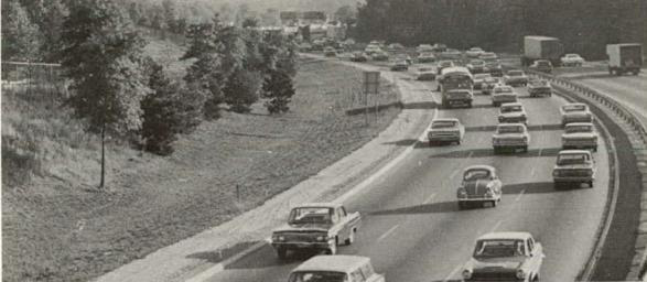
LOS E: LOS F: Unstable flow, operating at capacity, speed reduced, few gap for maneuvering, driver need to search gap, average spacing 33.5m (110 ft), v/c ratio ≈ 0.98 Forced or breakdown flow and low speed, demand exceed capacity, road in constant traffic jam.

Factors Affecting Capacity and LOS2074

• Roadway Factors: Lane width, Lateral clearance, Width of the Shoulder, Surface condition, Alignment and grade, Existence of road intersections
• Prevailing Traffic Factors: Directional distribution, % heavy vehicles

Passenger Car Unit (PCU)

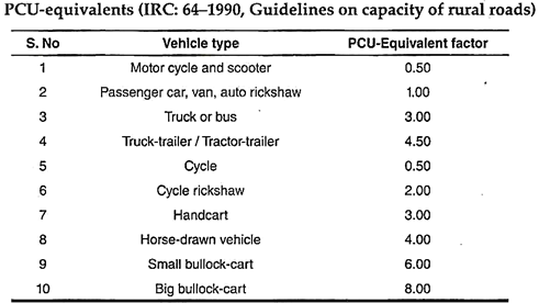
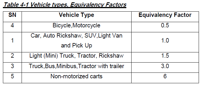
• In order to facilitate the estimation of traffic volume and traffic capacity while dealing with mixed traffic conditions, a common standard vehicle is chosen, and all other types are converted into this class of vehicle; passenger car.
• The passenger car unit (PCU) is the equivalent conversion unit for each vehicle type.
• The PCU represents the ratio of the minimum time or space headway consumed by a specific vehicle type to the headway consumed by a standard passenger car under identical conditions.

Factors Affecting PCU

• Vehicle Characteristics
• Transverse and Longitudinal Gaps
• Traffic Stream Characteristics
• Roadway Characteristics
• Regulation and Control of Traffic
• Environment and Climatic Conditions

Factors for Simple Analysis of PCU

• Average Speed
• Average Length and Width of Vehicle
• Average Transverse and Longitudinal Gap

Tasks

• Review basic traffic flow parameters
• Review relationship between speed flow and density
• Review capacity and LOS

1.6 Parking Studies

Review

• Traffic Capacity (Basic, Possible, Practical)
• Level of Service
• Factors Affecting Capacity and LOS
• PCU and factors affecting

Parking Study2073

• Parking is an act of stopping vehicles and leaving it unoccupied for certain period.
• A major problem in highway transportation in cities.
• Parking study is the study of existing parking facilities, their characteristics, demand and supply.
• Uses: Parking management and control, overall traffic control and transport policy implementation

Issues of Parking

• Reduction in road capacity leading to congestion
• Crashes during ingress and egress of parked vehicles
• Air and noise pollution due to stopping and starting of vehicles.
• Obstruction to emergency operation

Parking Management as Solution

• Parking affects mode choice.
• Good parking management and control can lead to
  • Higher car occupancies
  • Decrease in person trips
  • Greater public transport usage
  • Decrease in congestion and reduced air and noise pollution
  • Faster travel times and less travel delays

Parking Policies

• Parking policy affects how people will travel.
• Should coordinate with other planning objectives:
  • Design so that the street traffic is not adversely affected
  • Ensure complementary to the interest of business establishments along the street
  • Ensure complementary to public transport policies
  • Preserve the character of the neighborhood
• Peripheral parking schemes: Park and walk, Park and ride, Meet and ride

Types of Parking Facilities20822076

1. On Street/Kerbside Parking
2. Off Street Parking

On Street Parking

• Parking bays are provided alongside the kerb on one or both sides of the road
• Advantage: Convenient and requires less maneuvering
• Drawbacks: Reduce capacity, obstruction to traffic and high crash rate

Types:

• Parallel Parking
  • Preferred when limited space is available
• Angle Parking (30o, 45o, 60o and 90o)
  • Accommodate more vehicles but require more spacing
  • More convenient

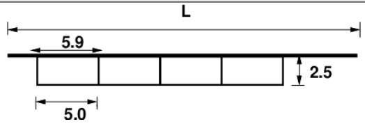
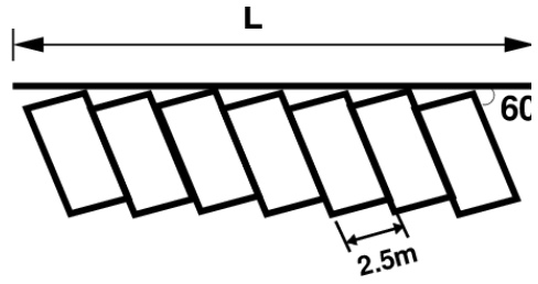
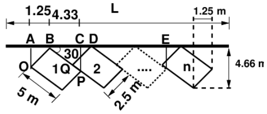
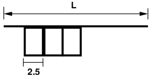
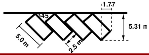
• On street parking should be prohibited near:
  • Intersection
  • Narrow streets
  • Pedestrian crossings
  • Special structures like bridge, tunnels
  • Entrance of buildings and houses

Off Street Parking

• Parking facility provided at a separate place away from the main stream of traffic
• Surface car park, multistorey car park, roof parks, mechanical car parks, underground park
• privately or publicly owned
• Advantage: No undue congestion and delay on the road
• Drawback: Some users have to walk greater distance

Off Street Parking: Surface Car Parks

• Provided on a piece of vacant land in front or surrounding an office, super market etc.

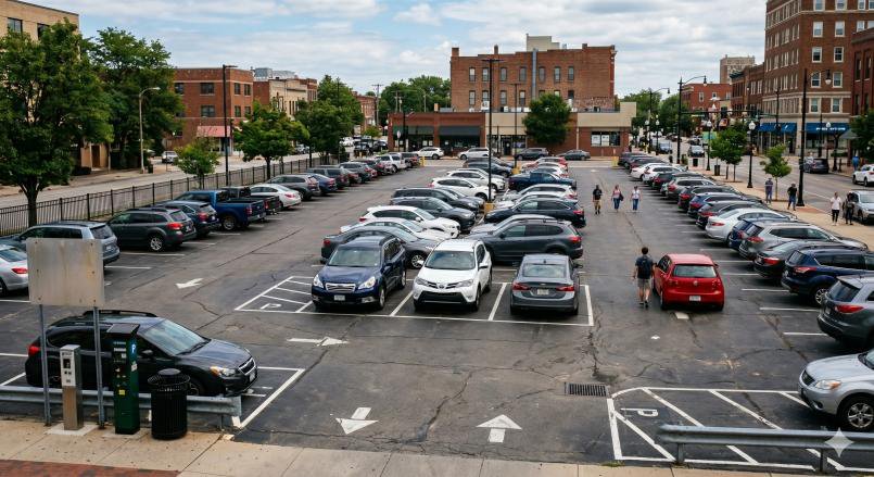
Off Street Parking: Multi Story Car Parks

• Parking space are provided in the different floor of the building which can be accessed through ramps or lifts.

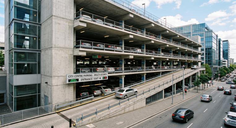
Off Street Parking: Roof Parks

• Park the vehicles on roof

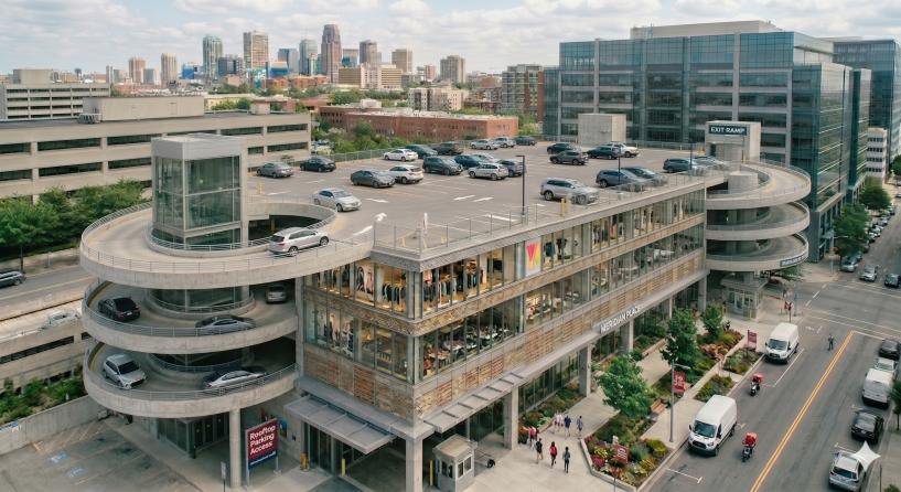
• Access ramps or mechanical lifts are provided to access roof

Off Street Parking: Mechanical Car Parks

• Mechanical lift to transfer cars to and from parking lots

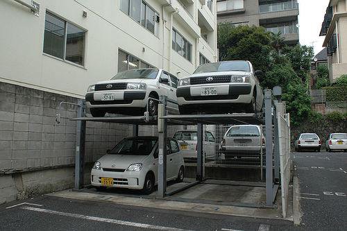
• Suitable where less space are available

Off Street Parking: Underground Parks

• Built in the basement of any building

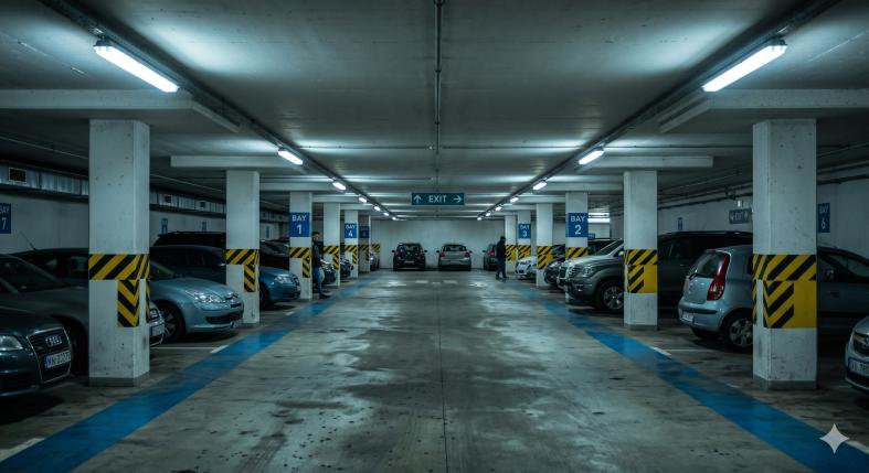
• Involves costly construction work of excavation, retaining wall, ventilation, lighting etc.

Parking Study

• Parking Characteristics Study
• Parking Inventory/Supply Study
• Parking demand Study or Parking Usage Survey (Cordon count: In-Out Survey, Fixed Period Survey, License Plate Survey; Questionnaire survey)

Parking Characteristics Study

• Present parking practices prevalent in the area
• The general problem in parking
• Interference to flow of traffic
• Records of crashes involved during parking and unparking operations if any.

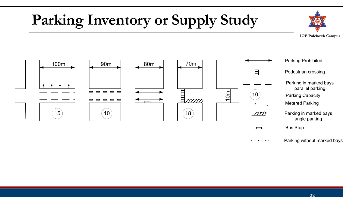
Parking Inventory or Supply Study

• The area under study is fully surveyed.
• A detail sketch of parking space inventory is prepared.
• Should include:
  • Detail information of all on and off-street features (Street layout, signals, bus stops, pedestrian crossings, length of kerb, unused land etc).
  • The existing situation of parking space inventory (parking capacity, parking prohibited area, public or private, control mechanism, fees and sensors if any)

Parking Demand Study or Parking Usage Survey

• Cordon counts
• Questionnaire Survey
• In-Out Survey
• Fixed Period Survey
• License Plate Survey

Parking Demand Study: Cordon Count

• Study area is demarketed with cordon line
• Vehicle entering and leaving area during different period of the day
• Parking demand obtained by subtracting the outgoing traffic from the traffic volume entering the cordon area.

Parking Demand Study: Interview Method

• Drivers of the parked vehicles, shop owners and other vehicle owners in the locality are interviewed.
• Detail information such as desired parking period of the day, preferred locations, frequency, amount of parking fee etc. are collected.

Parking Demand Study: In-Out Survey

• Initial count of parked vehicles is obtained at the beginning of survey.
• Then the number of vehicles that enter and leave the parking lot is counted.
• Parking load or occupancy can be obtained but parking duration cannot be obtained.

Parking Demand Study: Fixed Period Survey

• Initial count of parked vehicles is obtained at the beginning of survey.
• The count is again taken after a fixed interval of time (15min to 1hr).
• Chance of missing the vehicles parked for short duration.

Parking Demand Study: License Plate Survey

• The parking lot is monitored at continuous interval of 15 minutes or 30minutes and license plate number of vehicles in each bay is noted down.
• Parking duration and turnover can be also obtained.
• Labor intensive

Parking Demand Analysis

• Determine land demand for parking facilities
• Difficult task as various factors are interrelated
  • Growth in population and motor vehicle registration
  • Trends of CBD growth
  • Public policies regarding parking, public transit and pricing
• Parking attributes: Parking accumulation, parking volume, parking load, average parking duration, parking turnover and parking index

Parking Attributes

• Parking accumulation

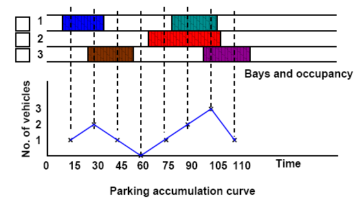
• Total number of vehicles accumulated in a specified area at a given time.

• Parking Volume
  • The actual number of different vehicles parked in a specified area over a given period of time. Usually measured in veh/day.
  • Does not account for repetition of vehicles
• Parking Load
  • It is total number of vehicle hours parked. Expressed as vehicle hours.
  • A measure of usage of parking space provided/demand.
  • Area under the parking accumulation curve

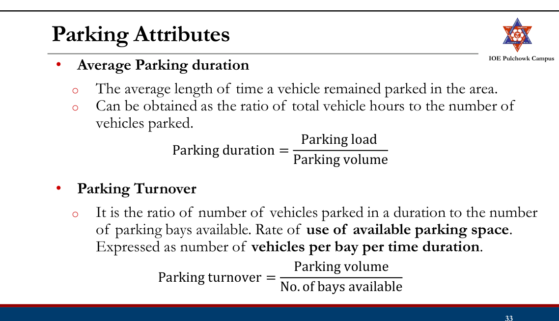
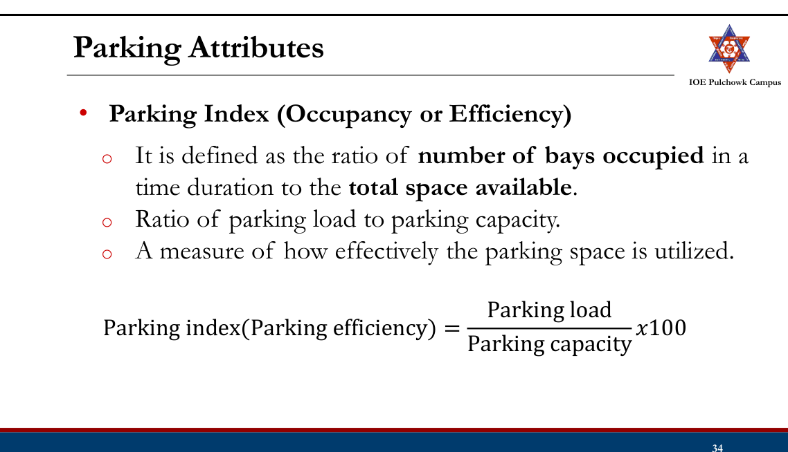
Parking Study

Example: From an in-out survey conducted for a parking area consisting of 40 bays, the initial count was found to be 25. The number of vehicles coming in and out of the parking lot for a time interval of 5 minutes is as shown in the table. Find the accumulation, total parking load, average occupancy and efficiency of the parking lot. Time In Out

Tasks

• Review parking studies, parking issues and management
• Review parking studies: parking characteristic study, parking inventory or supply study, parking demand or usage study
• Review parking demand analysis

1.7 Crash Studies

Review

• Parking issues, solutions, policies
• Types of parking
• Parking study (Parking characteristics study, parking inventory or supply study, parking demand or usage study: cordon count, interview method, in-out survey, fixed period survey, license plate survey)
• Parking demand analysis

Road Crashes

• Highways most problematic in terms of safety.
• 1.19 million deaths worldwide in 2021 alone from road crashes (WHO, 2023)
• LMICs most problematic.
• Nepal: Highest fatality rate in Asia, 28.2 deaths per 1 lakh populations (Asian Transport Advisory, 2025)

Crash Study20802070

• Study of traffic crashes trends, causes, and find out preventive measures to decrease numbers /severity of the crashes

Objectives of Crash Study:

• To study the causes of crash
• To evaluate existing designs and suggest corrections.
• To support proposed designs.
• To give economic justification for the improvements
• To compute financial loss.
• To carryout before and after studies

Causes of Crashes2075

• Road Users: Drivers, Cyclists, Pedestrians, Passengers, Animals etc.
• Vehicles
• Road and its condition
• Environmental such as Weather Conditions.

Causes of Crash: Road User Factors

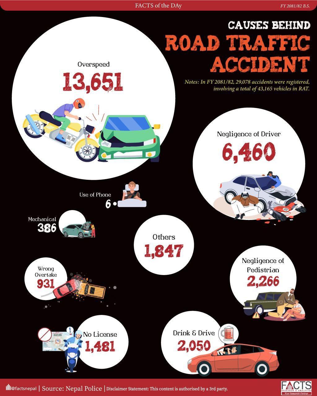
• Perceptual errors (failure to see or understand the traffic situation sign or signal due to lack of attention, distraction or distance)
• Lack of skill (inexperience, wrong action or decision)
• Manner of execution (aggressive driving, improper overtaking, carelessness, violation of rules and regulations)
• Temporary effects (alcohol, fatigue, drugs, sleep, illness, emotional stress)

Causes of Crash: Vehicles

• Defective tires and brakes, failure of steering system, lighting system etc.
• Lack of regular maintenance

Causes of Crash: Road and Its Condition

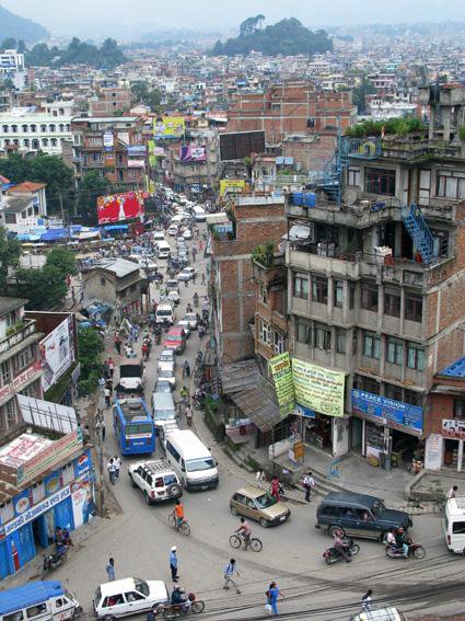
• Adverse road design (unsuitable layout and junction design)
• Adverse road surface condition (slippery, lack of maintenance)
• Inadequate/poor road markings and signs
• Unexpected obstruction (road works, parked vehicles)

Causes of Crash: Other Environmental Factors

• Unfavorable weather conditions
• Animals on the road
• Advertising boards

Crash Data Collection

• General: Date, time, persons involved and their particulars
• Classification: Fatal, serious, minor etc.
• Location
• Details of vehicle involved
• Nature of crash (vehicles involved, details of collision, pedestrian or objects involved)
• Road and traffic condition.
• Primary causes
• Crash cost

Crash Reporting

• Each crash should be reported to police.
• Crash report should include general, detail and other facts that might be useful in subsequent analysis and claims for compensation.

Crash Records

• Location Files
• Spot Maps
• Condition Diagram
• Collision diagram

Location Files

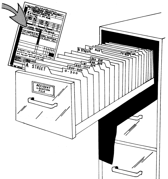
• File is maintained by location of the crash
  • A file is maintained for each intersection and midblock.
  • Then filed chronologically for each site.

Spot Maps

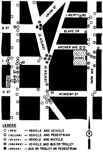
• Each time a crash report is filed, color-coded pin or other symbol is placed on a map at the appropriate location.
  • The color/symbol codes indicate the type and severity of the crash.

Condition Diagram

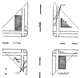
• A plan drawn to scale (1:100 to 1:250) showing all the important physical features at the crash location.
  • Aids the process of determining the causes of crash.

Collision Diagram

• The diagram consists of an

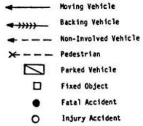
outline map of the location and symbols showing the direction of movement of vehicles/pedestrians/object s involved in crashes.

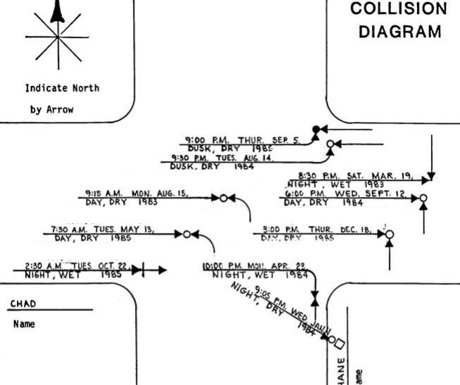
• Direction of travel.
• Date and time of accident.
• Road & weather conditions.
• Any unusual conditions (flood, storm, etc.)

Crash Study

Steps:

1. Obtaining crash data
2. Select high crash frequency locations

• Manually using location and spot maps or digitally based on crash rates

3. Conduct site analysis

• Detailed analysis of high crash locations using collision diagram and condition diagram for the locations

4. Summarize the facts (major collision types, potential causes)
5. Supplement with field observations
6. Analyze summarized facts and field data and suggest remedial measures

Crash Prevention

Measures:

• Engineering
• Enforcement
• Education

Engineering Measures

• Road Design and Maintenance: Checking & correcting geometric elements, checking road surfaces and providing maintenance measures, developing solutions to reduce conflict points
• Vehicle Maintenance: Routine checking and maintenance of braking system, steering, indicators, lighting system and tires
• Road Lighting: proper lighting especially at intersection, bridge etc.

Enforcement Measures

• Speed control
• Seat belts and helmets usage
• Traffic control devices (Heavy fine for violation)
• Strict testing before issuing license
• Medical checks (For vision, reaction time, drunk driving)
• Observance of laws and regulations

Educational Measures

• Educate road users about the traffic rules
• Education at school and universities about traffic safety
• Training course for drivers
• Traffic safety campaign (Films, documentaries, advertisement etc.)

Crash Analysis2073

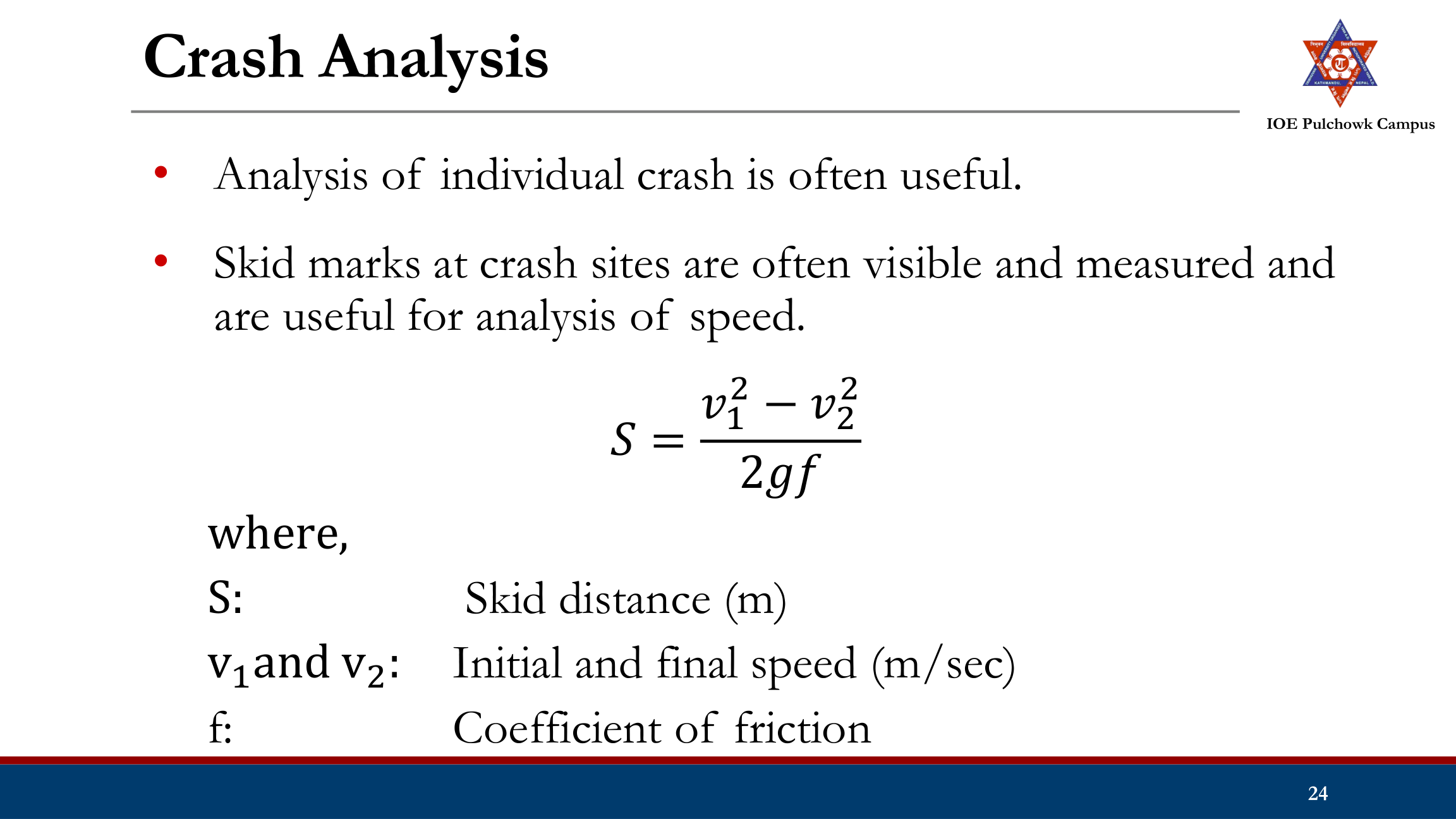
• Collision of moving vehicle with parked vehicle.
• Collision of two vehicles approaching from right angle

Collision of Moving Vehicle with Parked Vehicle2068

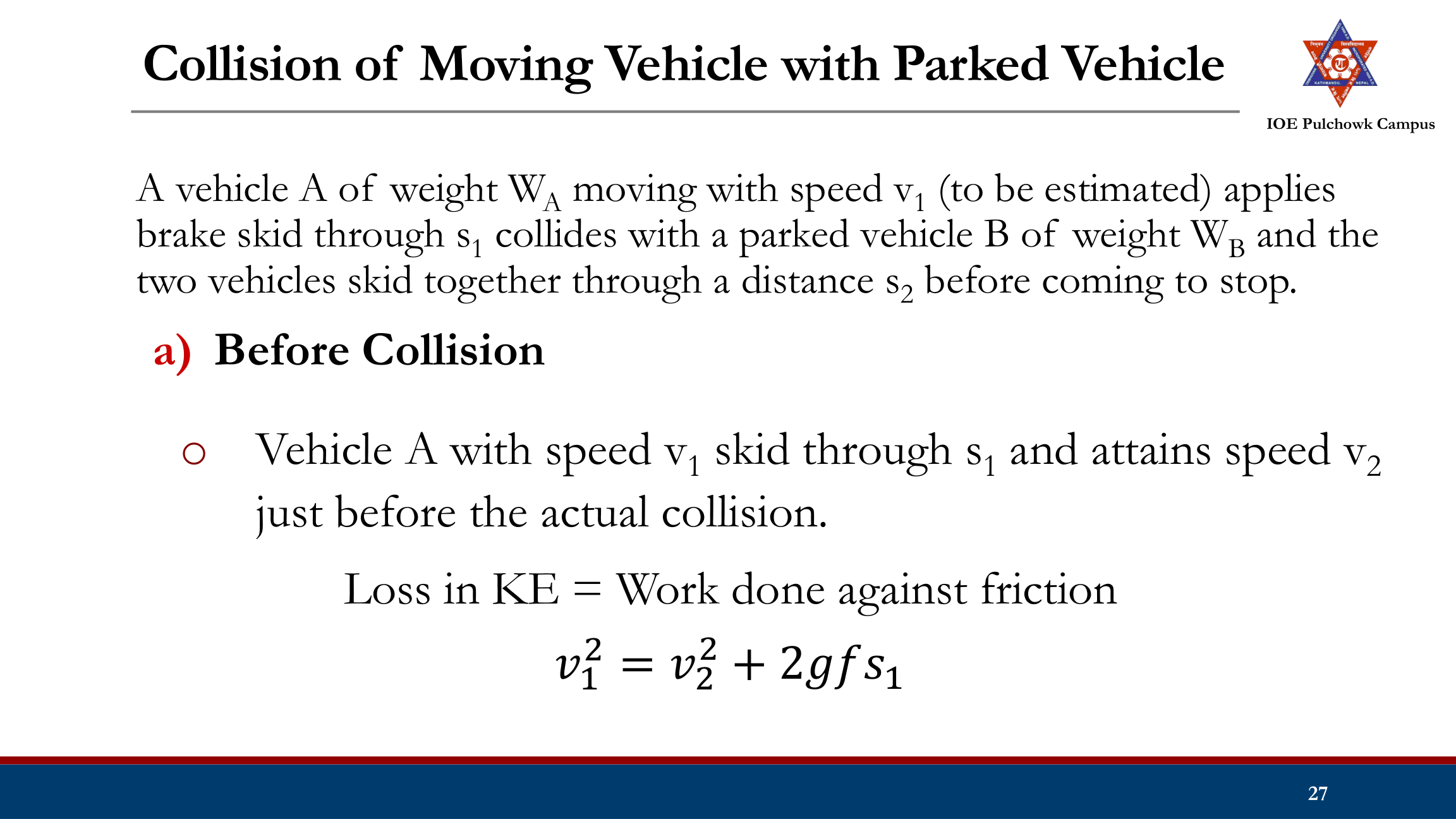
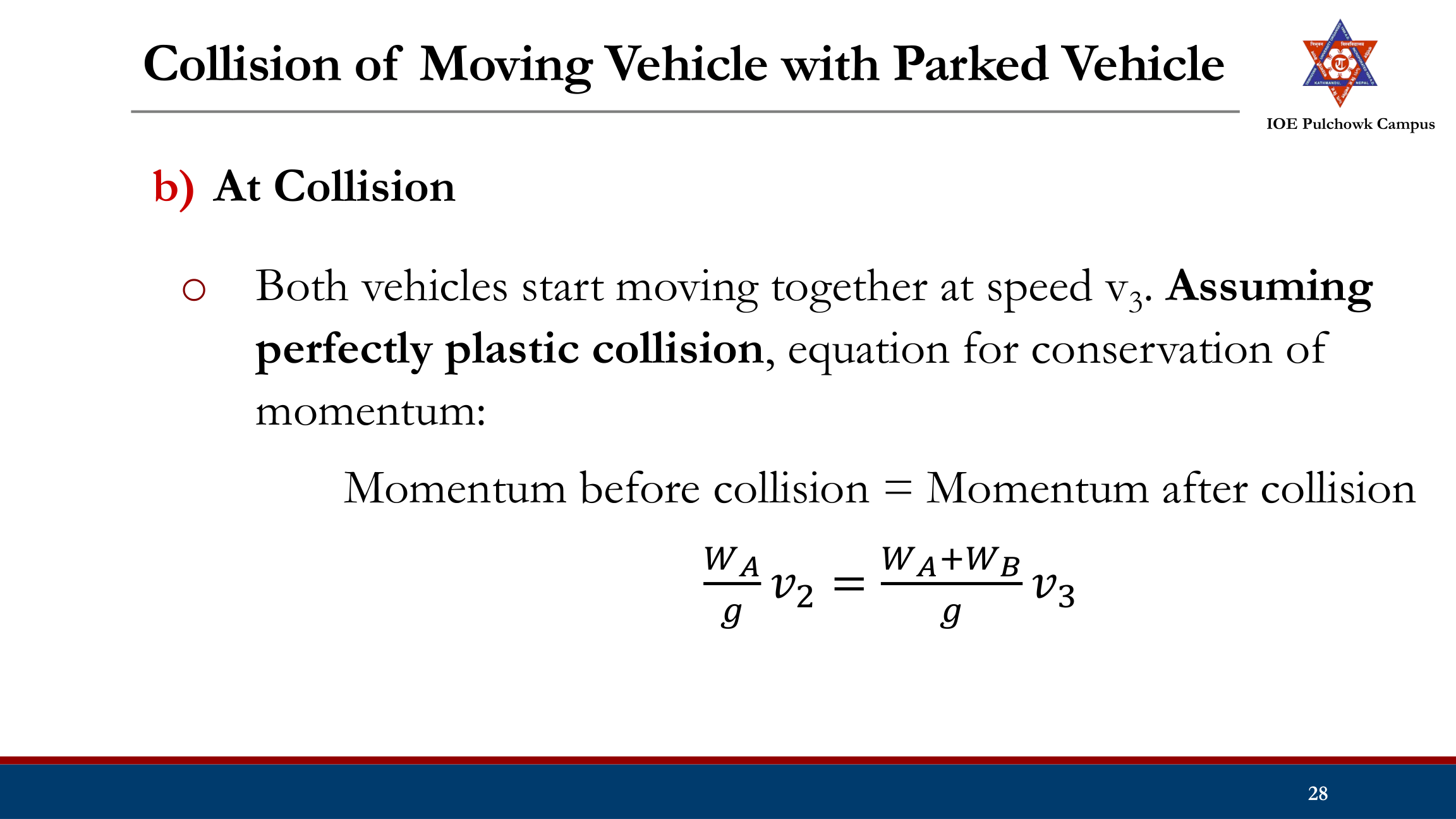
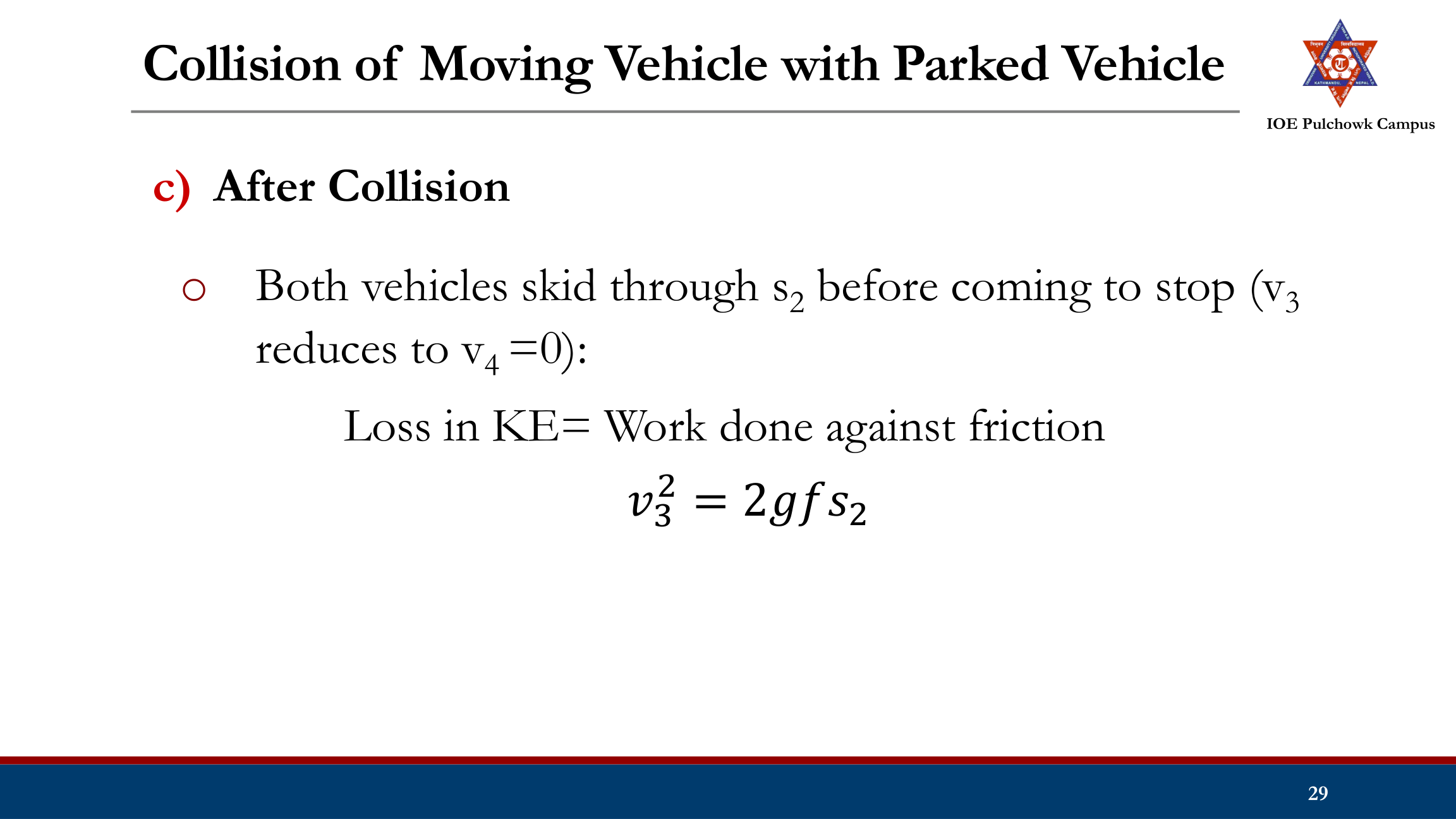
Crash Study

Example 1: A vehicle of weight 2 tonne skids through a distance equal to 40m before colliding with another parked vehicle of weight 1tonne. After collision both the vehicles kid through a distance equal to 12m before stopping. Compute the initial speed of the moving vehicle. Assume coefficient of friction as 0.5.

Collision of Vehicles Approaching from Right Angle2082208120802075

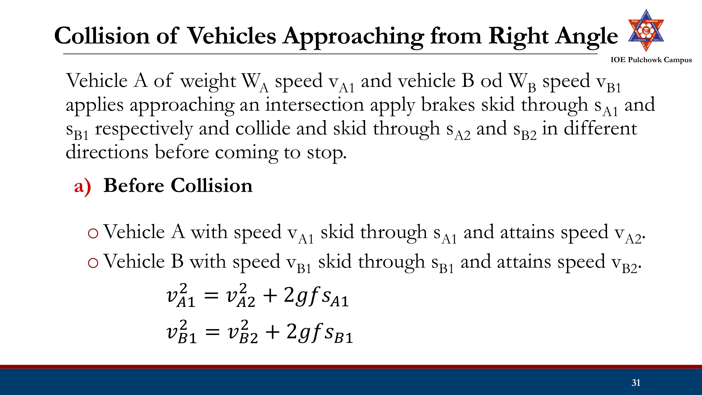
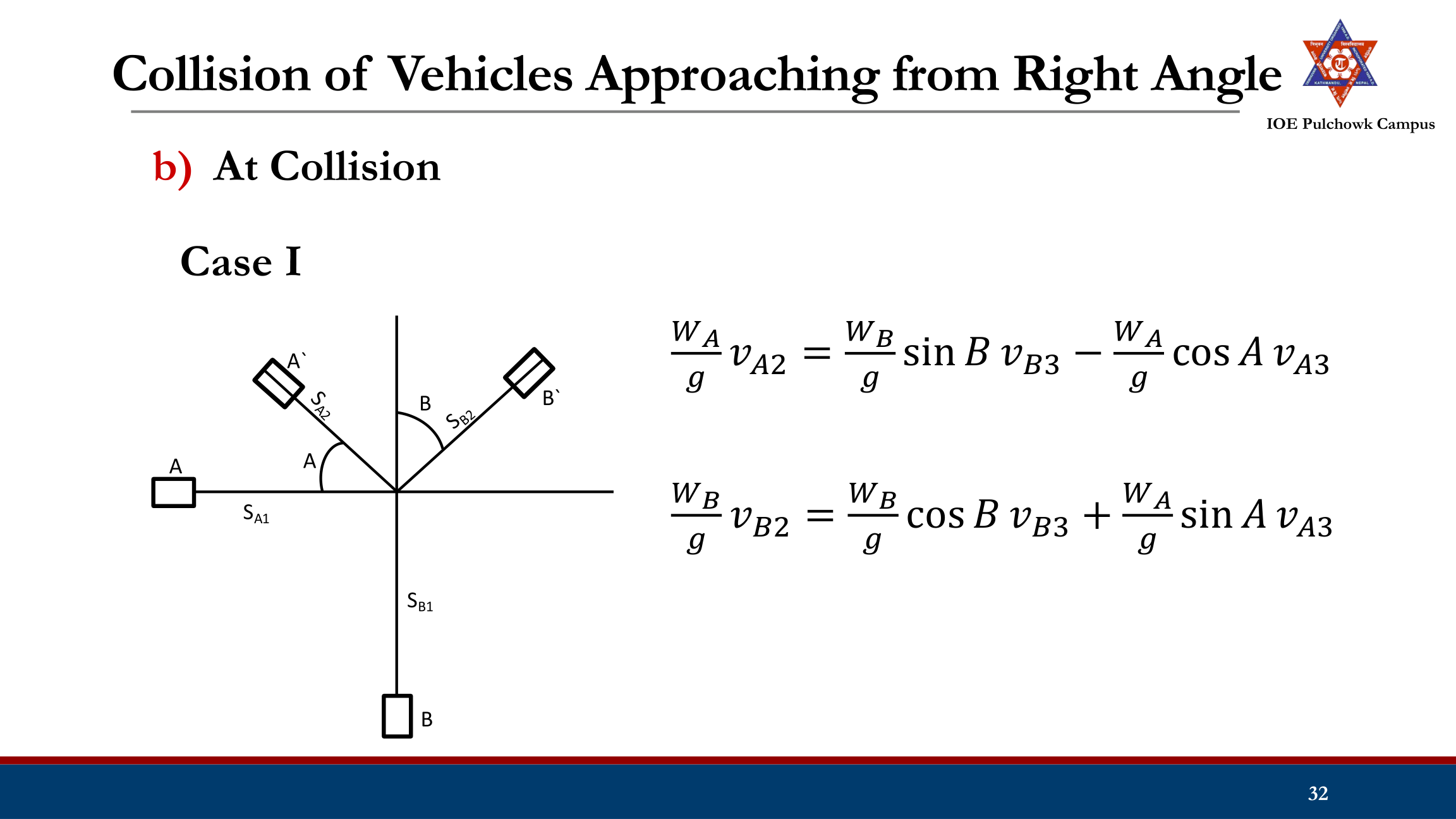
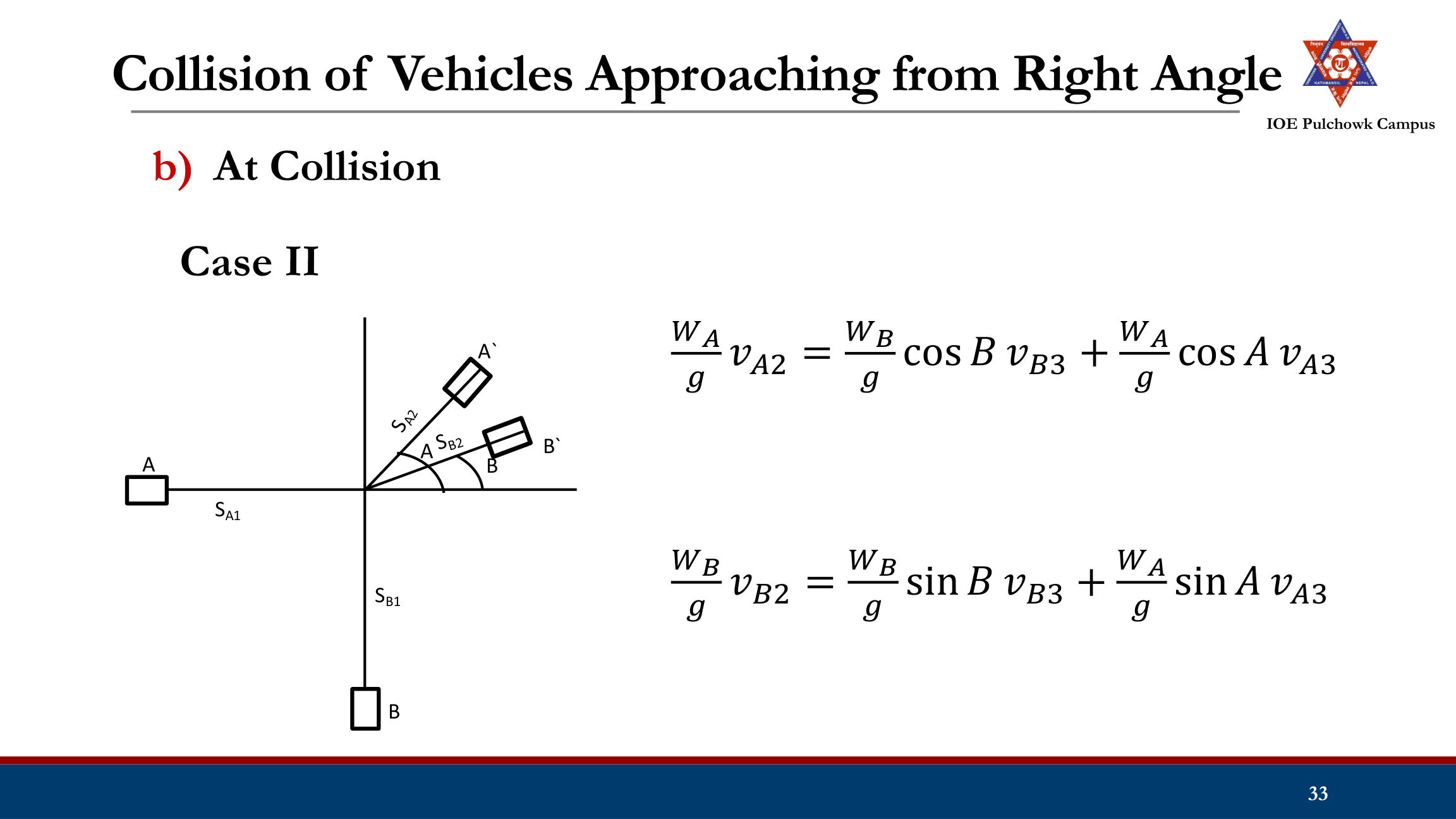
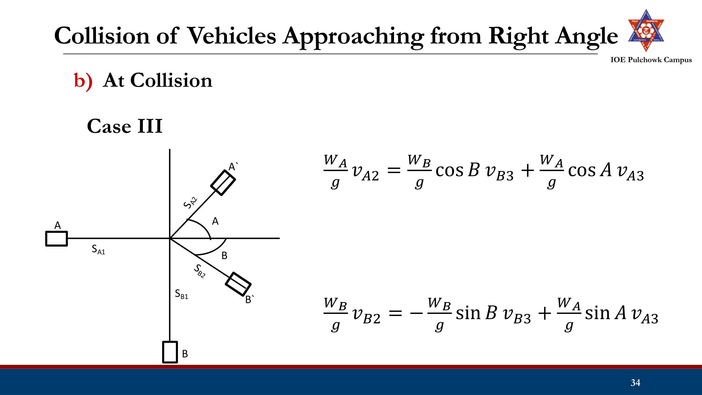
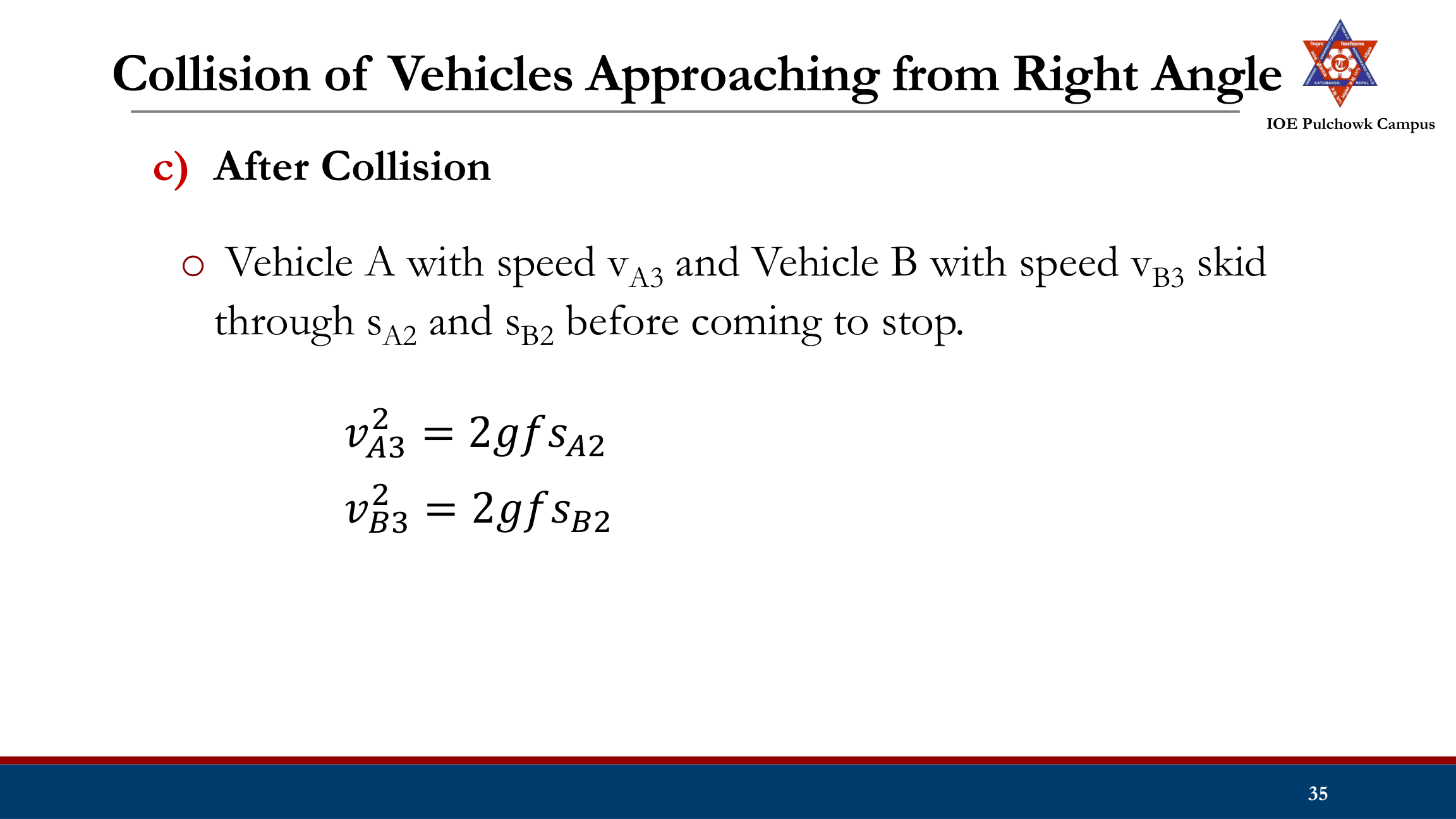
Crash Study

Example 2: Two vehicles A and B approaching at right angles, A from West and B from South collide each other. After the collision vehicle A skids in North direction 500 North of West and vehicle B 600 East of North. The initial skid distances of vehicle A and B are 38m and 20m respectively before collision. The skid distances after collision are 15m and 36m respectively. If the weights of vehicles B and A are 6 tonnes and 4 tonnes. Calculate the original speeds of the vehicles. The average skid resistance of the pavement is found to be 0.55.

Tasks

• Objectives of crash study, causes of road crash
• Crash data collection, reporting and records
• Crash study and crash analysis (collision of moving vehicle with parked vehicle, collision of vehicles approaching at intersection from right angle)

End of Chapter 1 — Traffic Studies and Analysis